Forces, Work, and Simple Machines

Formatted using: LyX 1.4.3, QCAD 2.0.5.0, and AC3D 6.5.28.

Forces, Work, and Simple Machines
Pamphlet to explain how simple machines work.
Online (soon) at http://www.math2learn.org/
Copyright (C) 2010 Michael Ward
michaelward@sprintmail.com

19 May 2010 : Advance Copy.
11 Dec 2011 : Corrections and clarifications.

This information is free; you can redistribute it and/or modify it under the terms of the GNU General Public License as published by the Free Software Foundation; either version 2 of the License, or (at your option) any later version.

This work is distributed in the hope that it will be useful, but WITHOUT ANY WARRANTY; without even the implied warranty of MERCHANTABILITY or FITNESS FOR A PARTICULAR PURPOSE. See the GNU General Public License for more details.

To receive a copy of the GNU General Public License visit http://www.gnu.org/licenses/ or write to the Free Software Foundation, Inc., 675 Mass Ave, Cambridge, MA 02139, USA.

For Jane and her kids.

Preface

Simple machines have been helping us work since before we could write. They help us move things more easily and achieve more than we could without them. They help us lift boulders, pry things apart, stack them together, transport objects and ourselves.

In order to understand a few of these simple machines and how they work we’ll use some basic math and physics (introduced as we need it).

My hope is that once you know what these simple machines are, and how they work, you’ll be able to see them at work in the world around you and put them to work for yourself. I also hope that once you see how easy it is, you’ll start to apply the same principles we use to understand these simple machines to other machines and even more complicated and subtle systems.

Acknowledgments

This pamphlet was inspired by Jane Kenney-Norberg and the LEGO Physics classes she developed and teaches at the Oregon Episcopal School in Portland Oregon where daily she inspires and helps develop the potential of hundreds of children with benefits that increase with the more I learn about her programs, education, and development of the human brain.

Special thanks to Jane, Jimmy Springer, Kristen Haferbecker, the engaging, curious, and delightful LEGO Physics students and Teaching Assistants for giving me a chance to be a part of it all.

I’d also like to thank Leo Rice and Asher Klatchko for ideas for some of the exercises.

Table of Contents

Chapter 1: Forces

Chapter 2: Work

Chapter 3: The Lever and Fulcrum

Chapter 4: The Wheel and Axle

Chapter 5: Rope and Pulley Systems

Appendix A: Simple Equations

Appendix B: Vectors

Appendix: References and Recommendations

1 Forces

One of our main concerns will be the movement of an object from one location to another. In order to move an object we’ll apply either a push or a pull. Since we’ll be talking quite a bit about these pushes and pulls, we’ll use the technical term from physics, and call each push or pull a force. Forces are what move things around in the world. We owe this idea to Issac Newton who lived hundreds of years ago (from 1642 to 1727). He figured out rules for how forces make things move. There are three basic rules that that make up Newton’s Laws of Motion. In very basic language, the first two laws can be stated as:

Without forces, things remain in a constant state of motion. If they are already moving, they keep moving in the same direction and at the same speed. If they are not moving, they stay put.
Forces cause things to change their motion in the direction of the force. The more force, the bigger the change.

Newton’s laws of motion opened the door to understanding why objects fall to the ground and why the moon orbits the earth. Of course, you probably already know I am talking about the force called gravity. In honor of figuring all this out, forces are often measured in units named after the person who gave us this insight: Newtons (abbreviated as N). However, since we are just getting started with forces and trying to build up our intuition, we’ll start with a more familiar unit of force: Pounds [A] [A] You may wonder about kilograms at this point. However, there is a subtle distinction between kilograms (which are units of mass), and pounds (which are units of force). This becomes important with careful use of Newton’s second law, but in practice we can convert between pounds and kilograms with an appropriate assumption and conversion factor. See, for example, chapter 1 of my “Introduction to Rocket Science: How high will it go?” (abbreviated as Lbs). Since approximately 4.48 Newtons is equal to one pound, one Newton is approximately 0.223 pounds, about halfway between a quarter and a fifth of a pound: 0.223 ≃ 1 ⁄ 4.48.

You probably already have experience measuring some quantities like length, weight, and temperature that can be captured by a single number. However, forces are a bit more complicated than this. To see why, let’s start with temperature. Imagine a room with a light-bulb on in the middle of it. Since the light-bulb functions as a source of heat, we expect that temperatures near the light-bulb are higher than than temperatures farther away. If we had some sort of instant-read thermometer, we could move it throughout the room, reading the temperature at various points.

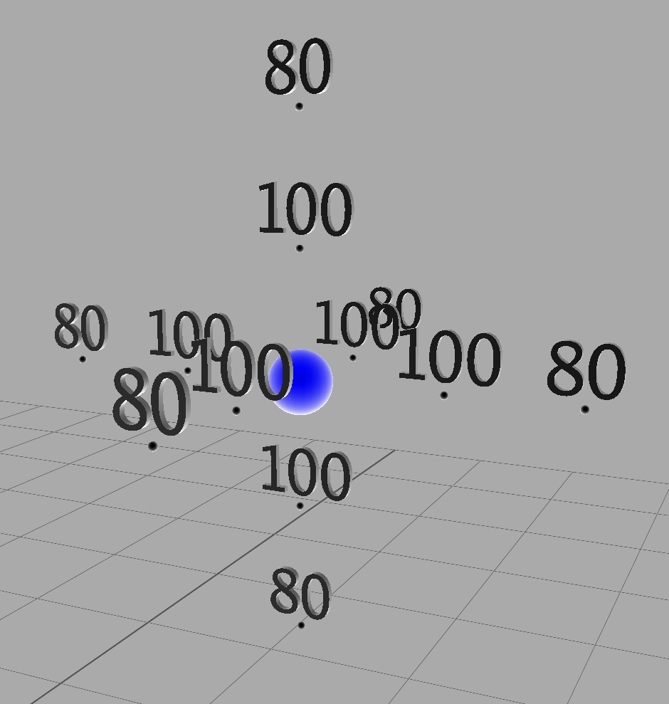
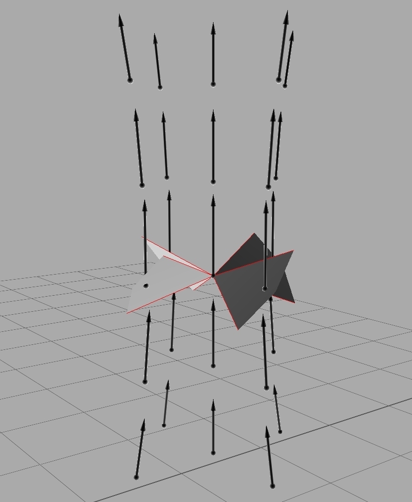
Now let’s imagine a comparable scenario for forces. Imagine a similar room with a fan instead of a light-bulb. As the fan spins, it pushes the air around in the room. As the air presses on things, it exerts a force. One way to measure the force at a point in the room would be (without disturbing the air flow) to release a small soap bubble at that point and observe its change in motion at that point. We would have to measure two different things about the motion. We would have to notice both how quickly it started to move and the direction in which it started to move. One of the most versatile ways to represent such a measurement is with an arrow. The tail of the arrow is placed at the measurement point, the tip of the arrow points in the direction of the motion, and the length of the arrow indicates the how quickly the motion changed at the measurement point. These arrows form a mathematical system of vectors, and there is a whole algebra of adding, subtracting, (several ways of) multiplying, and even dividing vectors [B] [B] For a quick introduction to vectors see AppendixB↓..

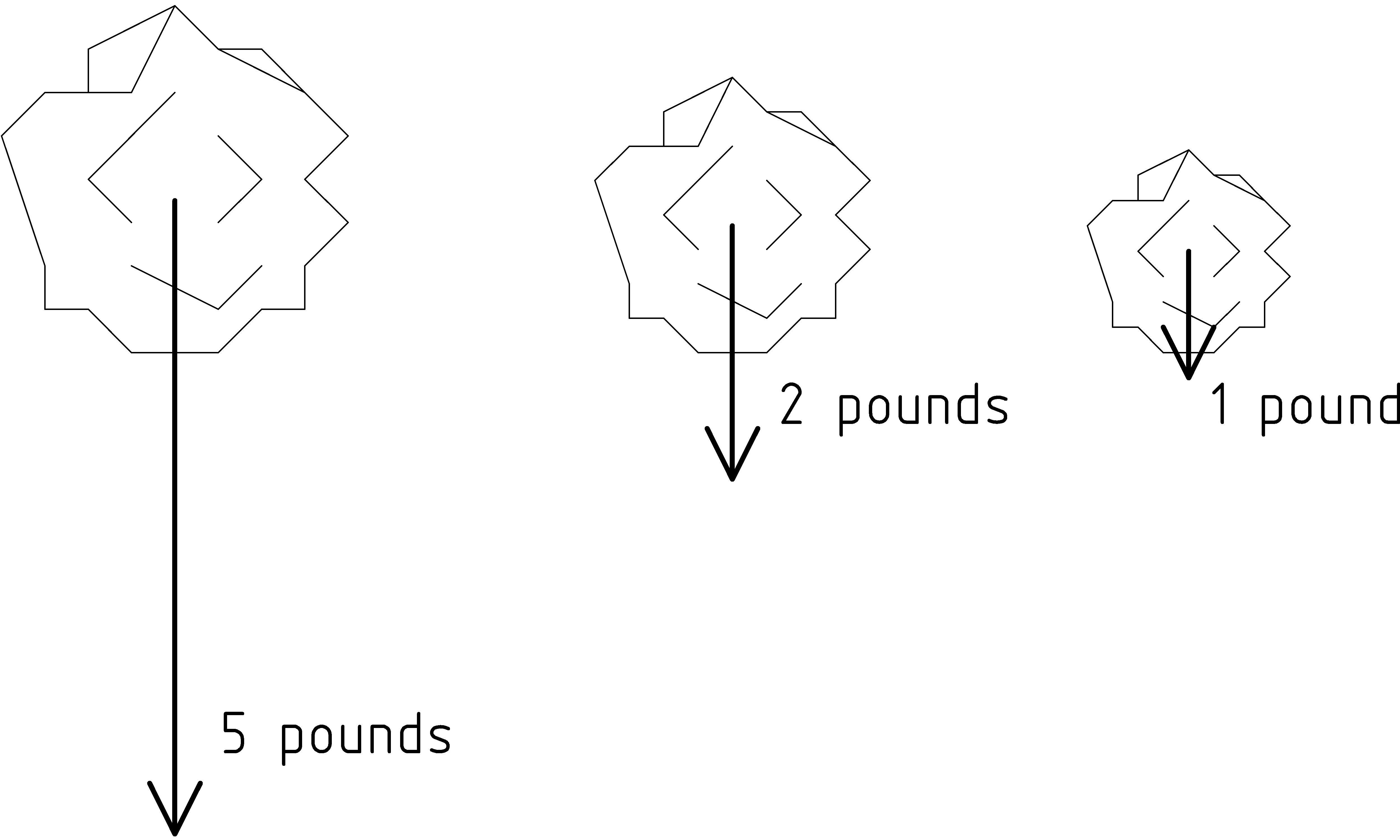
Let’s try this out with a force that we are all familiar with, the one generated by the very planet on which we live, the earth’s gravity. We’ll consider the force of gravity on three stones, one weighing 5 pounds, one 2 pounds, and a 1 pound stone, each being pulled down toward the ground by different amounts. You can feel the difference if you try to lift them. The 5 pound stone is harder to lift: it is the heaviest. We can measure the force on each of the stones with a weight scale. If our scale is accurate and measures weight in pounds, the 5 pound stone will weigh ... 5 pounds. The force of gravity will pull the stone down against the spring of the scale until the needle [C] [C] If you are using a digital scale, the stone pushes down against the pressure sensor and the electronics either flip through digits or wait until readings stabilize enough to read 5.0. points to 5. The 2 pound stone will be pulled down a little less than half of that, until the needle reads 2 pounds. The 1 pound stone will be pulled down against the spring exactly half as much as the 2 pound stone. The direction of the force in each case is straight down, toward the center of the earth. To draw the vectors for the force on each stone, we’ll first draw the arrow down from the 1 pound stone with a convenient size for the arrow. Then the arrow for the 2 pound stone will be twice as long, and the one from the 5 pound stone will be 5 times as long.

We could have used different sized arrows, but it is a good idea whenever possible to use the same scale for all the vectors in the same diagram. For example, if the stones weighed 50, 20 and 10 pounds instead of 5, 2, and 1 pounds, we could use the same diagram, using the same arrows to represent the forces (except different labels) because 20 pounds is just 2/5ths of 50 pounds, just as 2 pounds is 2/5ths of 5 pounds. (See exercise 1↓.)

Now, let’s use this concept of force to consider [D] [D] An experiment we perform only in our minds is known as a thought experiment and performing them is a proud tradition in physics, though using your mind to figure things out only by thinking about them is not unique to physics and is a generally a good idea ;^) a 20 pound stone sitting still on the ground. We know gravity is pulling down on the stone. If forces make things move, why is it just sitting there not moving? You probably already know the rock doesn’t move because it is on the ground, and the ground is firm and doesn’t budge much even when you jump on it. Let’s change the way we are thinking about it.

We can think of the ground pushing up on the stone, just like gravity is pulling it down. In fact, we think of the ground pushing up on the stone just exactly as much as gravity pulling down on the stone, so that the two forces on the stone are in opposite directions but have the same magnitude, canceling each other out. We say that the sum of the forces is zero. The pressure to move down is exactly canceled by an upward pressure in a way that is similar to the way that a motion 3 feet to the north is canceled by a motion 3 feet to the south. When we add the two motions together we end up right where we started.

The case of adding two vectors of the same length, but opposite directions is one of the simplest examples of adding vectors. Let’s take a look in the following diagram:

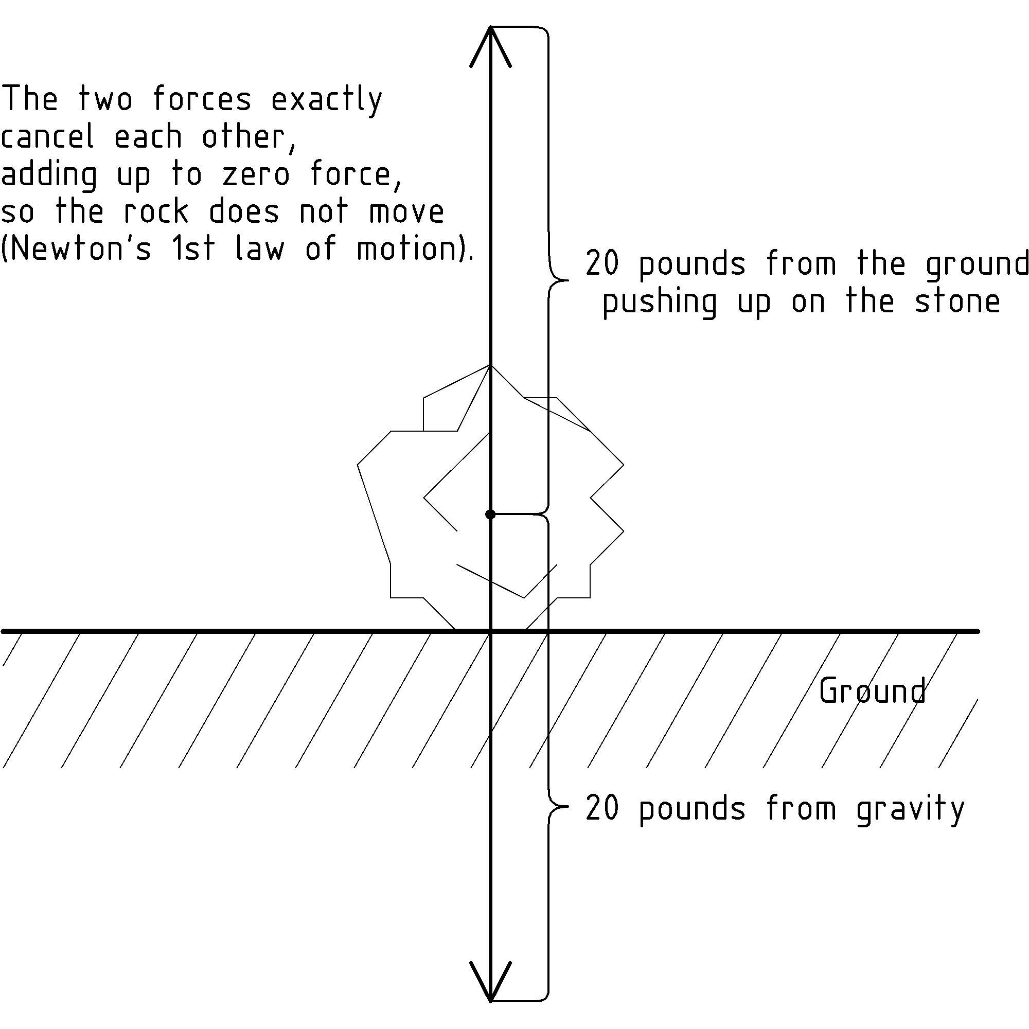
More generally, when two vectors lie on the same line we simply add their signed magnitudes, where we pick one direction of the line as positive and the other as negative. In our case we can pick up as positive and down as negative so that we have -20 pounds of force from gravity and +20 pounds of force being supplied by the ground. When we add them together we get a resulting force of 0 pounds so that, by Newton’s 1st law of motion, the rock stays put. (For more on adding vectors, see appendix B↓.)

Now, let’s continue to use this concept of force to consider what happens when we lift the 20 pound stone up from the ground onto a picnic table. We bend down (with our legs, not our backs), extend our arms and put our hands underneath the stone on both sides so that everything will stay balanced (so the stone doesn’t fall as we lift it), grab the stone, and then we start to lift (with our legs). We start to apply force with our leg muscles. To be most effective (to use the force of our leg muscles most efficiently) we lift straight up, directly countering the force of gravity that is pulling the stone straight down. (We’ll talk more about force, the direction of motion, and resulting work in the next chapter).

If we lift very slowly, gently increasing how much strength we use, at first nothing happens except that we feel increasing pressure in our hands and legs. Increasing the use of our muscles slowly, we feel the stone move up and away from the ground just at the point at which we apply exactly as much force up as gravity is pulling the stone down. As we put more muscle into it, the stone moves up more quickly. This is Newton’s 2nd law of motion: as the resulting sum of forces becomes greater, the stone increases its motion in that direction. As we gently decrease our effort, the rock comes to a stop with us (instead of the ground) pulling up on the rock just enough (20 pounds worth) to counter the pull of gravity.

Before we move on to consider the work done when we move objects around, try your hand at the following exercises to test your understanding so far.

Exercises

Make a diagram with two stones: a 6 pound stone sitting on a table, and 3 pound stone that is just beyond the edge of the table, at the height of the table, falling toward the ground (as if it has just been pushed off the table). Draw arrows to represent the forces on both the 3 pound, and the 6 pound stone.
Think about the situation where we are starting to lift a 20 pound stone up, off of the ground. Suppose that we start lifting with 5 pounds of force, and the rock is not yet moving. With how much force must the ground still be pushing up against the rock to exactly counterbalance the remaining gravitational force? Make a diagram with the rock on the ground and the 3 force arrows that summarize this situation: one force arrow for gravity, one for your 5 pound lift, and the third for the push of the ground. Draw all of the arrows with their tail as a dot at the center of the stone. Be sure to label the arrows as in the diagram back on page 1↑.
Suppose that you weight 100 pounds and that you can easily walk up stairs and jump up and down.
1. At a minimum, how much force can you generate with both legs?
2. Suppose that both legs are equally strong. At a minimum, how much force can one leg generate?
3. Suppose that you can jump up and down on only one leg. At a minimum, how much force can that one leg generate?
Just as 2 piles of 5 beads is 2 × 5 = 5 + 5 = 10 beads, and 3 groups of 4 is 3 × 4 = 4 + 4 + 4 = 12, 2 times 1/5th is 2 × (1)/(5) = (1)/(5) + (1)/(5) = (2)/(5) = (2 × 1)/(5). More generally, we have in a similar way, for any integers n, m, and non-zero d: m × (n)/(d) = (n)/(d) + ⋯ + (n)/(d) = (m × n)/(d). Similarly, (n)/(d) × m = (n)/(d) + ⋯ + (n)/(d) = (m × n)/(d). Use this along with the fact that the denominator d of the fraction represents division by d to find the integer value for 2/5ths of 50: (2)/(5) × 50 = ?

2 Work

We already have some intuition about work from what we feel when we move things (including ourselves) with our bodies. In this chapter we’ll use this together with the idea of forces from the last chapter as a guide to help us generate a definition of work. This will help us gain a deeper understanding of work, including a surprising result about something that feels like work, but won’t count toward the way we measure it.

You probably know when you’ve done some work, say, lifting a 20 pound stone from the ground up onto a table. You can feel in your legs (if you are lifting properly) that you’ve done some work. You’ve applied a force to the rock and moved it some distance, say 2 feet. How much force was applied? 20 pounds of force. Until you apply 20 pounds of lift to the stone, it stays put. Once you balance the downward force of gravity exactly with an upward directed force to cancel it, the stone is free to move in an upward direction with an application of additional force in that direction. In this chapter, we’ll quantify (figure out how to assign numbers to) the amount of work using mathematics you probably already know.

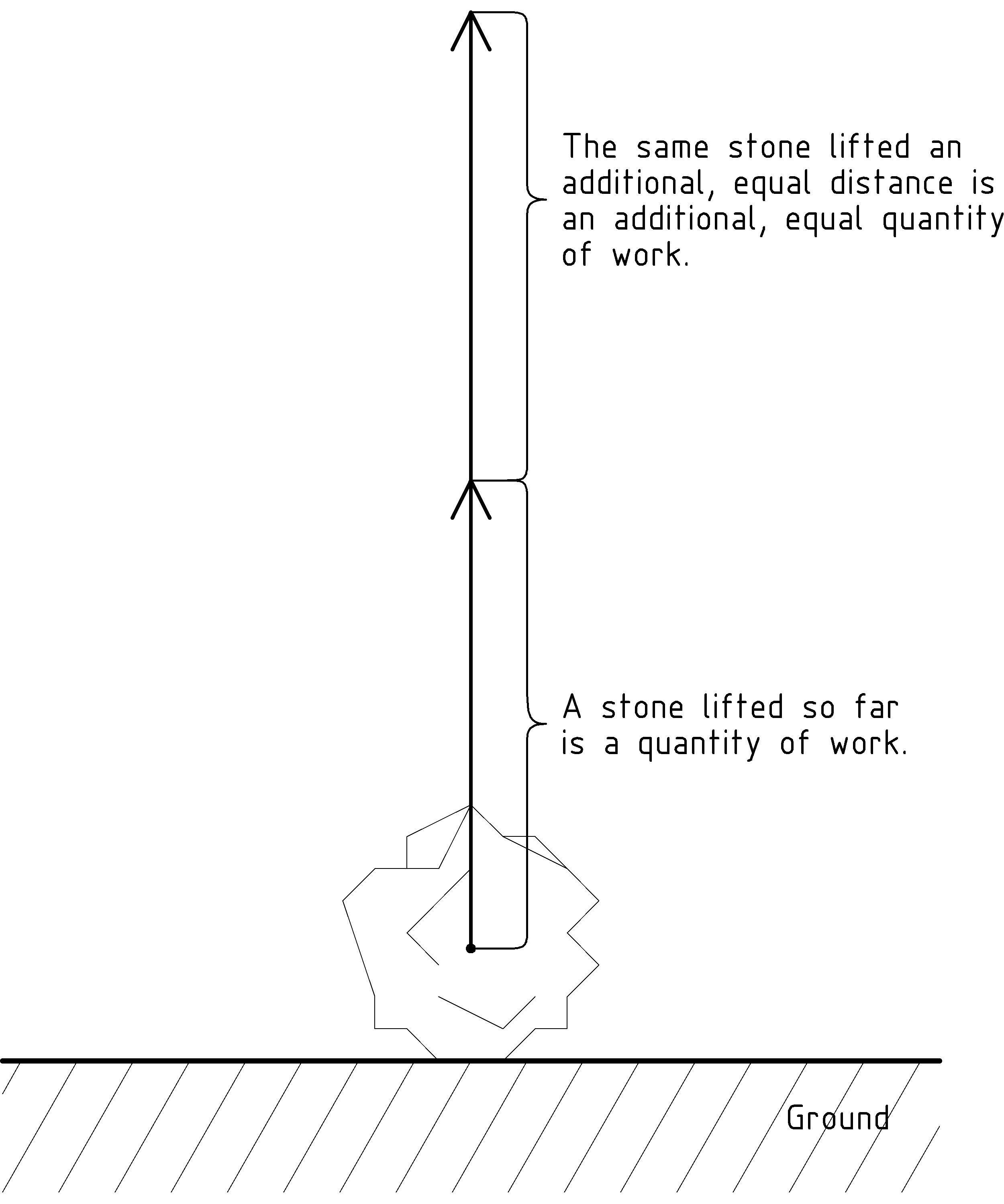
We start with a couple of simple observations. First, we’ll want to arrange things so that if we lift the stone twice as high, we’ve done twice as much work. Similarly, if we lift the stone only half as high, we’ve done only half as much work. We can capture this in a mathematical expressions by multiplying by the distance that we’ve lifted the stone so that we have, so far:

Work = (some math expression) × Distance

Multiplication by distance captures this aspect of work nicely. If we lift something three times as far, we’ve done three times as much work. We’ll have more to say about direction and distance later, but before we take a closer look at that, let’s include a second observation in our mathematical definition of work.

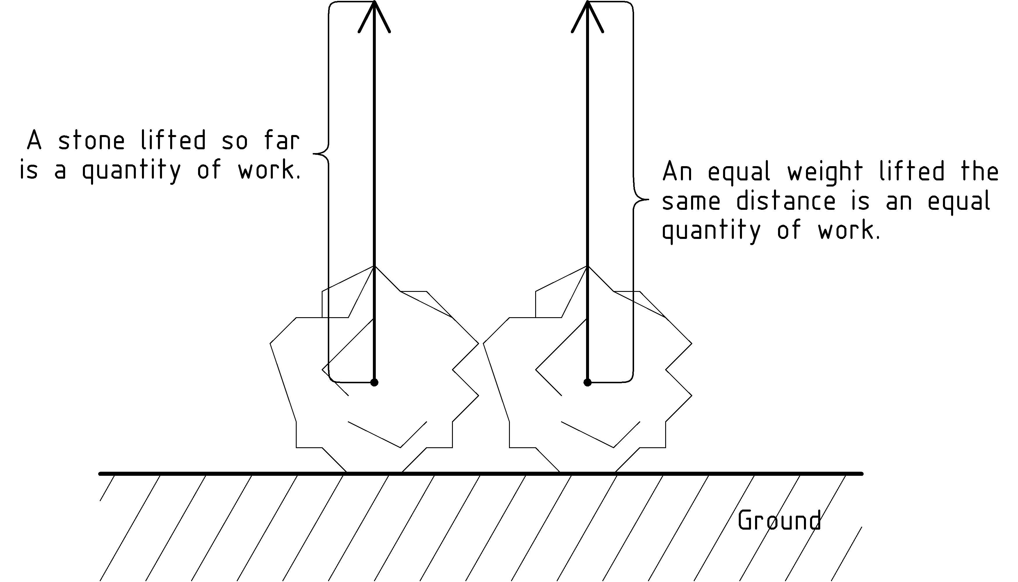
The second observation we’ll want to capture is that if the stone weighs twice as much (think of it as split into two equal parts), and we lift it the same distance, we’ll again have done twice as much work. Similarly, lifting a stone that weighs only half as much requires only half as much work. To finish off our mathematical definition of work, we have to combine this with the downward gravitational force of the stone from the last chapter. In particular, to lift the stone, we exert a force on the stone that counters the gravitational force causing the stone’s weight. From our perspective, the work we’ve done in lifting the stone is the following multiplicative combination of not only how far we’ve moved the stone, but also the amount of force we’ve had to apply to move it:

Work = Force × Distance

We’ll call this the work equation and we’ll use it to find numeric values for work. So, for example, in lifting a 20 pound stone 2 feet we do 40 foot-pounds worth of work. Lifting a 10 pound stone 3 feet requires 30 foot-pounds of work.

Here comes the surprising part of our definition. What if we push on a really heavy boulder sitting on the ground, one that weighs, say, 1000 pounds, without moving it? Since the distance moved is zero, we haven’t done any work even though it feels like it. However, if we think about it the right way, this makes sense: even though we may push really hard against the boulder, we haven’t really accomplished any work, even though we may use a significant amount of energy trying. This reflects the fact that with our quantitative definition of work we are measuring results external to ourselves, in the world, not internally, how they feel inside.

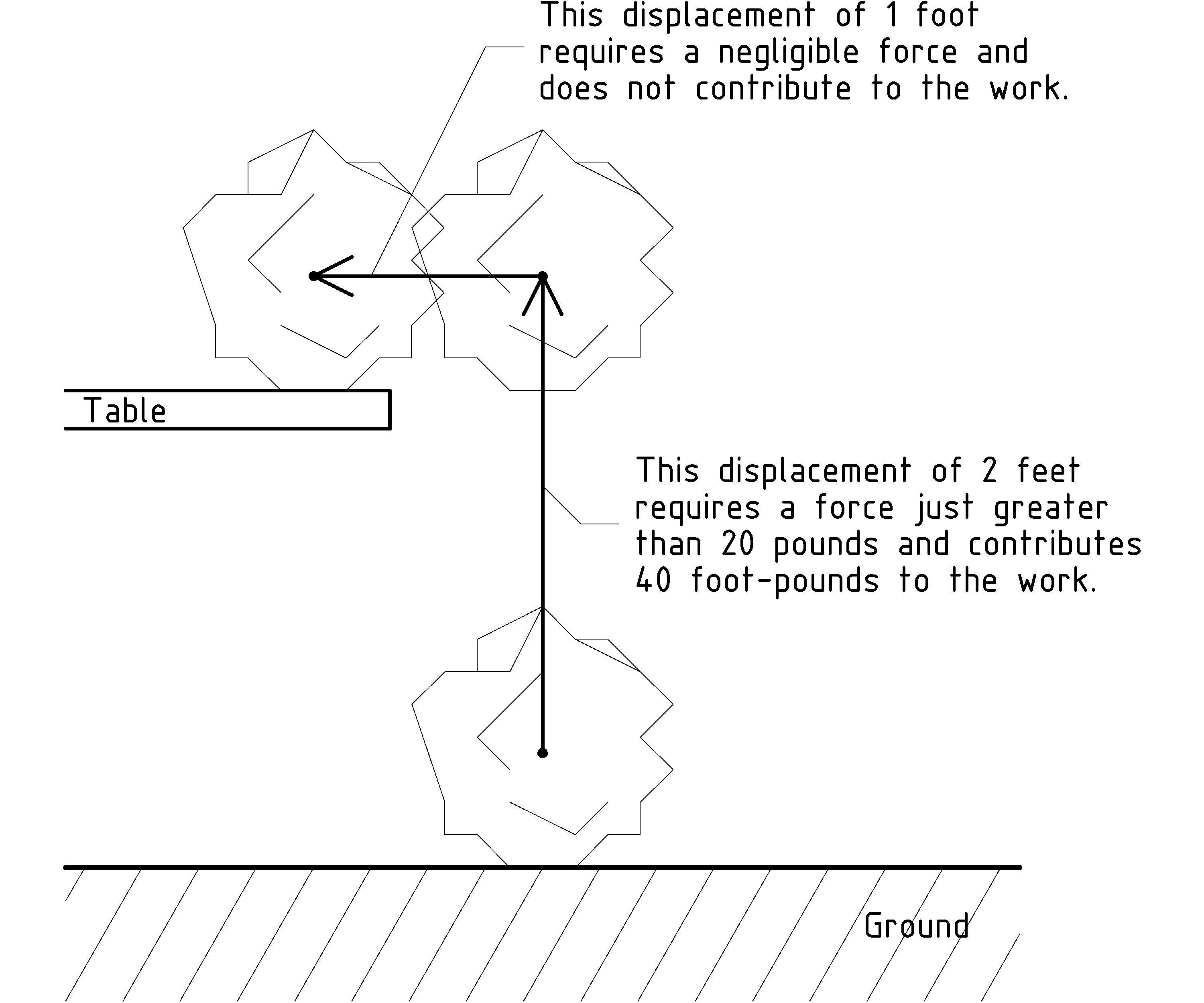
Now, let’s continue with our example, thinking about lifting a 20 pound stone 2 feet to set it on a table. In addition to lifting the stone, there is a force and distance required to move it over to the table top:

This brings up a number of interesting questions about the kinds of work done in lifting the stone and setting it on the table. The first distinction we make is between conserved and unrecoverable work. Conserved work is work that is stored in some way that allows recovering the work. For example, in lifting the stone from the ground to the table height, we have stored the work in the height of the stone. We could get 40 foot-pounds back out of this configuration, by letting the stone fall through the 2 feet, back to the ground, perhaps lifting something else as it falls. The potential work that is stored in the height of the stone is called potential energy.

What about once we’ve lifted the stone, and are just holding it up without moving it? Just as with the 1000 pound boulder sitting on the ground: even though we are spending energy to keep the stone at the height (it feels like work), according to our definition, since the stone is not moving (distance is 0), we are doing no work.

Next let’s consider the horizontal motion of the stone required to set it on the table top. First we consider the horizontal motion through the air with no [E] [E] I should say “essentially no resistance” because there is some resistance just to push the air out of the way. However, for our purposes, we will consider this exceedingly small amount of work insignificant. Can you think of a situation in which pushing the air out of the way is so much work that we must take it into account? resistive forces. We use Newton’s second law of motion that tells us: without some force to cancel it, even the tiniest force on the stone in the direction of the table top will cause the stone to start moving in that direction. We’ll leave figuring out exactly how much force and how fast the stone moves to a more advanced investigation of Newton’s laws [F] [F] For example, if you’d like to get involved with model rocketry, check out my pamphlet “Introduction to Rocket Science: How high will it go?”. In this pamphlet, we’ll simplify the situation to say that, in principle, we could make the sideways force, and thus the work, as small as we’d like. In this case we can ignore completely this non-resistive horizontal motion of the stone. However, just so that you can know about the other kinds of work and energy, we’ll briefly consider the other cases.

So, on the other hand, suppose that we pushed hard, increasing the stone’s motion in the horizontal direction so much as to do a significant amount of work. This work would also be stored, in this case, in the horizontal motion of the stone. This is called kinetic energy. We can recover the work by having the stone hit or push something, performing some work for us, perhaps, storing it as potential energy with some ingenious mechanism (such a spring and catch, or the lifting of some weight).

The final kind of work is unrecoverable. Unrecoverable work is work that is lost and cannot be recaptured. This sort of work can arise from sliding the stone along the table top. The configuration of the table top surface with the stone pushing down on it causes the two surfaces to stick together. The amount of stickiness depends strongly on the nature of the surfaces and creates an opposing, resistive force to our push called friction.

Consider an air-hockey table (providing a slippery cushion of air) with the bottom of the stone being smooth, flat, and large enough to keep the stone floating. Then the tiniest push will start the stone sliding. In this case there is almost no force opposing a push and we say that there is (practically) no friction. Moving the stone 1 foot could take an insignificant amount of force (and thus work), just like moving it through the air.

On the other hand, if the table has a rough, wooden surface that creates a significant amount of friction, we might have to push with 5 pounds of force in order to slide the stone. In this case, the frictional force opposing a push is 5 pounds, and in sliding the stone 1 foot across the table we would do 5 foot-pounds of work. What happens to the work? Is it stored somewhere? It is, actually. The rough surfaces rubbing together create heat.

You can try it with your hands. Try rubbing the palms of your hands against each other, back and forth, while pressing them strongly together. The harder you press your palms together, the more friction you create, and the more heat you generate. Furthermore, the faster you rub your palms together, the more friction you create, and the more heat you generate.

In general we can’t recover the work that creates heat. The subject that deals with the study of heat, heat transfer and storage, and exactly how (and how much) heat can be converted into work is the area of science known as thermodynamics that we’ll leave for some future investigation.

Exercises

Fill in the empty cells in the following table:

Force(A)/(A)	Distance	Work
12 pounds(A)/(A)		36 foot-pounds
(A)/(A)	4 feet	36 foot-pounds
5 pounds(A)/(A)	3 feet
6 Newtons(A)/(A)		12 Newton-meters
7 Newtons(A)/(A)	3 meters

Suppose we have two ways to lift a 12 pound stone 2 feet. How much force must be applied to lift the stone directly? How much work is done? An easier way requires only 6 pounds of force. If the amount of work is the same, over what distance must the 6 pounds of force be applied?
Imagine being at the top of a steep hill on a bicycle.
1. Coasting down the hill on the bicycle converts what sort of energy into what sort of energy?
2. When you apply the brakes, what sort of force are you counting on?
3. If the brakes are working well, what sort of energy is created?
For this exercise, let’s suppose that all 100 pounds of your weight is located at the center of your body. Suppose that when you crouch down to jump as high as you can, the center of your body is at a height of 1 and 1/2 feet, and that at full extension your center is at a height of 3 and 1/2 feet. Further suppose that during the jump your legs can apply a force of 200 pounds to lift your body through the jump when you are trying to jump as high as possible.
1. What is the displacement of the center of your body for the portion of the jump during which your legs apply the force?
2. If you are trying to jump as high as possible (using the full force that your legs can supply), what is the work done by your legs for this portion of the jump?
3. What is the minimum work required to lift your body for this portion of the jump?
4. What is the difference between the the minimum work required and the work done by your legs when trying to jump as high as possible?
5. At the point your feet leave the ground, what sort of energy stores the extra work done by your legs identified in part (2↑). Will this energy continue to do work? Does it influence the height of the jump?
6. To what height do you expect the center of your body to travel by applying 200 pounds of force with your legs?
In this exercise [G] [G] Thanks to Asher Klatchko for the ideas behind this exercise., suppose that all 100 pounds of your weight is located at the center of your body. Suppose that your jogging stride is 4 feet, and that with each jogging stride you move your center of weight up only 1/2 foot. Assume that you jog efficiently by not jumping during the stride, so that your foot stays in contact with the ground for the complete upward motion of your body, and any time spent cruising through the air is in the forward and downward direction. (In other words, assume that most significant part of the work of the stride is spent lifting your body the 1/2 foot.)
1. How much work is done with each jogging stride?
2. Estimate the work done in running one mile (5280 feet).
3. Without changing your weight, name two ways to increase your jogging efficiency (decease the work required to jog a mile).

3 The Lever and Fulcrum

In this chapter we take a look at what must surely be one of the simplest and first machines ever used by humans. We probably first used these machines before we started writing stories to preserve knowledge across generations. To make one of these simple machines, all you need is a strong stick to use as a lever, a rock for a fulcrum, and then you are ready to use it to tumble a boulder. Let’s take a look at the basic configuration and name the essential parts [H] [H] Thanks to Jane Kenney-Norberg for this diagram.:

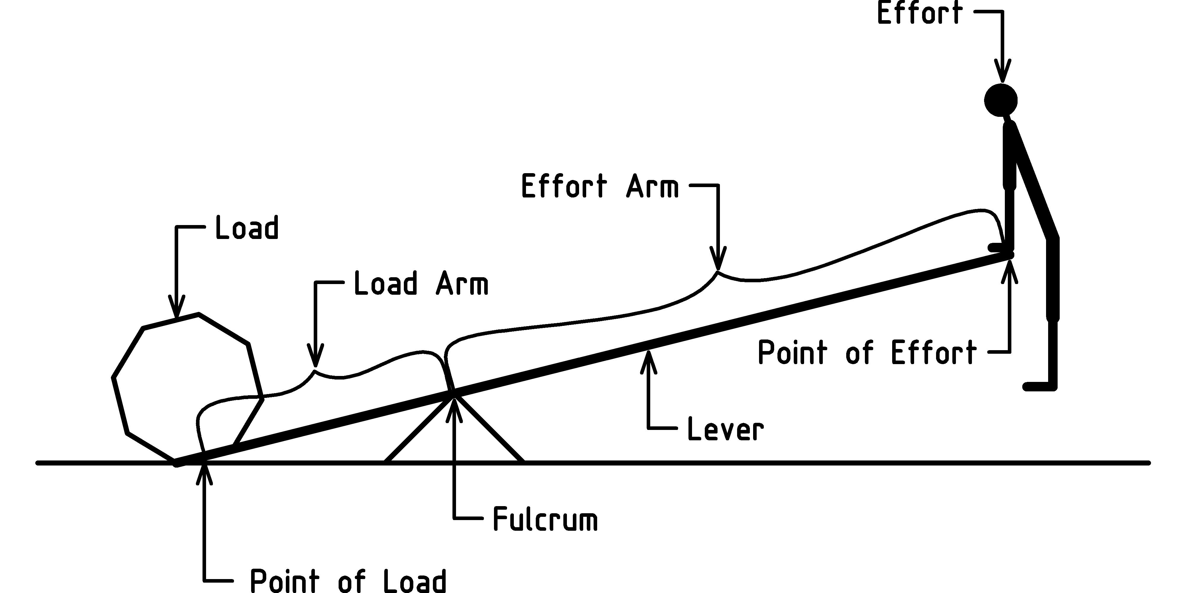
There are two fundamental parts of this simple machine: the lever, and the fulcrum. An ideal lever is straight and strong. This allows the full transfer of force from the point of effort to the point of load. An ideal fulcrum comes to a point and is immovable (however, in practice a sharp point is easier to break and can damage the lever more easily than a rounded point). The lever is composed of two parts, the load arm and the effort arm. The load arm is the part of the lever that extends from the fulcrum to the point of load (where the load is located on the lever). The load is the object to be moved or pushed against. The effort arm is the part of the lever that extends from the fulcrum to the point of effort (the position where force or effort is applied to move the load).

To see how a lever and fulcrum make lifting an object easier, let’s take a look at a specific case: lifting a 24 pound rock, 1 foot, using a 12 foot lever. Let’s place the fulcrum so that it divides the lever into a 4 foot load arm, and 8 foot effort arm:

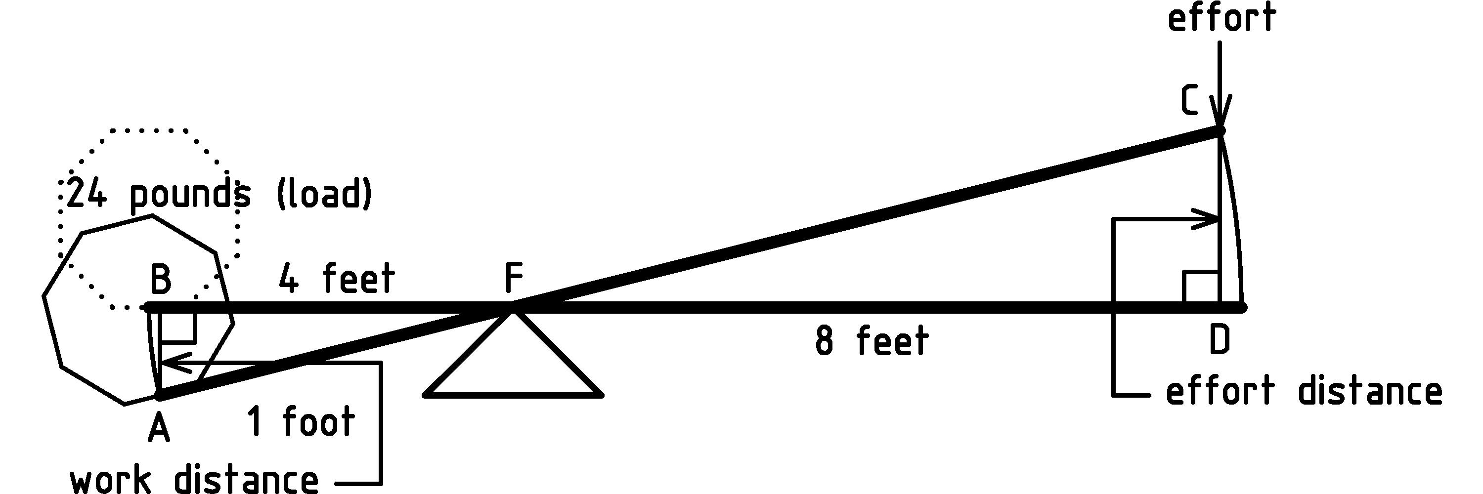
Let’s label the points of the load triangle ABF and the effort triangle CDF. I’ve placed small squares at the corners B and D to indicate those corner angles are the same as that of a square (they’re called right angles) indicating that the work distance and the effort distance are vertical. More to the point, the work distance is along the line of gravitational force (weight) that the rock feels and so, as we discussed in chapter 2↑, we can use the work equation to determine the amount of work in lifting the rock as:

Work = Force × Distance = 24 pounds × 1 foot = 24 foot − pounds

To further our understanding, we’ll ignore any friction at the fulcrum or bending of the lever, and make the assumption that the work done in lifting the rock is the same whether we lift it directly, or use the lever and fulcrum. This is what is known in physics as a conservation principle, a rule that says that some quantity remains constant across some sort of change. In our case, work is constant across the change of how we perform the work. We can say that work is conserved or talk about the conservation of work in simple machines. We can use this to better understand the effort side of the situation, but first we’ll need a little geometry.

We need to observe that triangle ABF has the same shape as triangle CDF. In other words, the corresponding angles of the triangles are the same [I] [I] When two geometric objects have corresponding angles that are the same, we say the objects are similar. When the objects have the same angles and size, we say they are congruent. Rather than saying two line segments, angles, or triangles are congruent, Euclid would have said “equal.”: the angle at A is the same as the one at C, the angle at B is the same as the one at D, and the angles at F are the same. (For more on this see exercises 3↓ and 3↓.) This means that the effort triangle and its parts are some multiple of the load triangle and its parts [J] [J] Another way to say this is that the two triangles are in proportion: dividing corresponding lengths gives the same ratio. That ratio is the scale factor, or multiple, mentioned in the text. This is a combination of Euclid Book I propositions 28 and 29 about angles of parallel lines, and Book VI proposition 2 about cutting a triangle with a line parallel to a side.. This allows us to work out the scale factor, since we know the lengths of the load and effort arm are 4 feet and 8 feet respectively:

Load_Arm × Scale_Factor = Effort_Arm 4 feet × Scale_Factor = 8 feet

We can see that the scale factor is 2 in two ways: either by figuring out what we have to multiply 4 feet by in order to get 8 feet, or by dividing both sides of the equation by 4 feet (see Appendix A↓ for more on working with equations). Either way, we know that the effort triangle and its parts are 2 times bigger than the load triangle and its parts. This means that the effort distance is 2 times 1 foot, or 2 feet. Let’s take a look at how this configuration makes it twice as easy to lift the rock.

To lift the rock up, we push straight down on the effort end of the lever so that the lever rotates about the fulcrum. We push down through the effort distance of 2 feet. We now use the work conservation principle to reason that the amount of work in lifting the rock with the lever is the same as lifting it directly. Since we know how much work it is to lift the rock directly, 24 foot-pounds, we can now use the work equation to figure out how much effort we have to apply to the effort arm to lift the rock:

Work = Force × Distance 24 foot − pounds = Force × 2 feet

This tells us that we only have to use 12 pounds of force to lift a 24 pound rock! It is twice as easy to lift the rock with the lever and fulcrum! A lever with an effort arm twice as long as the load arm has magnified our strength by a factor of 2. However, notice (diagram page 1↑) that in order to lift the Load (24 pounds) the Work_Distance (1 foot), we had to apply the Effort (12 pounds of force) through the Effort_Distance (2 feet) so the amount of work remains the same. This is the assumption we started with. Let’s be even more explicit with the following lever-work equation :

Load × Work_Distance = Effort × Effort_Distance

What we are really counting on to make sense of all of this is that the work on the left side of the equation is the same as the work on the right side. Even though we have good reason to believe the work is the same, how can we check that it really works this way? Exercise 3↓ may give you an idea for some experiments you try to test this equation. However, let me just say that the more accurate your measurements of distances and weights, the more important the weight of the lever itself becomes.

We need to look at one more aspect of the effort force before we move on. You may want to review the discussion of the horizontal motion on page 1↑. We found there that we could ignore the force to move the stone horizontally, that the work of moving stone to the table top was due almost entirely to the force of lifting the stone straight up.

Similarly, with our lever and fulcrum, only the force in the direction of the work distance contributes. Because of the geometry of the lever and fulcrum, this translates directly into the force we apply through the effort distance. Only the part of the force we apply to the lever straight down contributes significantly to the work of lifting the 24 pound rock. This is why we use the vertical distances rather than the curved arc lengths in the lever-work equation: the vertical distances lie completely in the direction of the force needed to lift the rock.

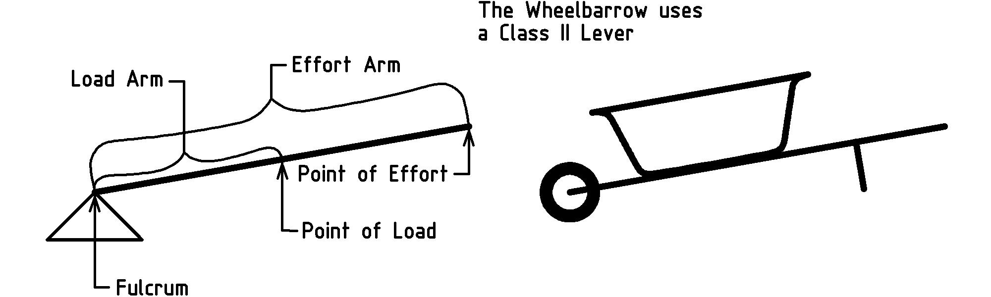
Lever and fulcrum machines are so useful and have been applied in so many ways, that their configurations have been categorized into classes [K] [K] http://en.wikipedia.org/wiki/Lever. The diagrams on pages 1↑ and 1↑ show what is known as a class I lever [L] [L] To be used as a lever and fulcrum simple machine, a lever is always paired with a fulcrum. However, our human nature to collapse blocks of information into more compact abstractions often causes us to abbreviate the phrase “lever and fulcrum” to the shorter, single word “lever”.. The effort arm and load arm occupy different portions of the lever on opposite sides of the fulcrum. In class II levers, the load and effort arms overlap, occupying a common portion of the lever, with the point of load between the fulcrum and point of effort:

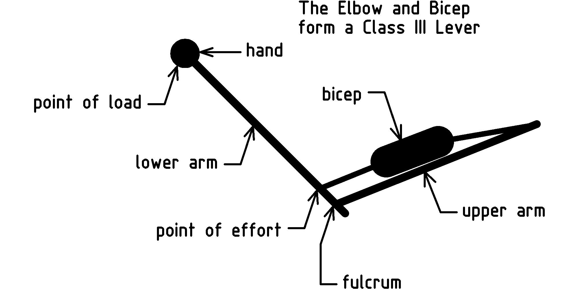
Class III levers have the point of effort positioned between the fulcrum and the point of load. The most familiar example of a class III lever is the elbow and bicep of the human arm:

In addition to these lever classifications, I’ll give you one final configuration that utilizes a pair of levers, connected with an axle or freely rotating connection that functions as a fulcrum for both levers. These simple machines are so handy, that not only have you probably already used them, but you probably don’t even think twice about how they work:

One thing all these different lever configurations have in common is that the same principles that we used to understand the class I levers apply: the similarity of the load and effort triangles, and the conservation of work. Exercises 3↓ and 3↓ give you a chance to work with these other configurations.

We can even use levers in a purely abstract way as described in appendix A to help us better understand concepts, or even to calculate the area of curved geometric shapes as Archimedes did thousands of years ago [M] [M] See Netz and Noel’s “The Archimedes Codex: How a Medieval Prayer Book is Revealing the True Genius of Antiquity’s Greatest Scientist” for this fascinating story. One of the recovered writings described is the method wherein Archimedes uses the leverage principle (see the leverage equation on page 1↓) to calculate the area of a parabola section, foreshadowing our modern conception of the Calculus..

Finally, there is a specialized application that is so profound that it is considered its own, distinct simple machine. We’ll take a look at this more closely in the next chapter, but first, try the following exercises to test and improve your understanding of lever and fulcrum systems.

Exercises

The first two exercises ask you to write and work with some equations. If this sort of thing is new to you or you feel like you want to know more about equations before trying this, see Appendix A↓ first.

Euclid’s Definition 10 in Book I of a right angle tells us that the angle of any line is composed of two equal angles (like the corner of a page) called right angles and Postulate 4 of Book I tells us that all right angles are equal. If we assign numeric measures to angles so that a right angle measures 90 degrees (90^○), this tells us that the angle of a straight line is 180 degrees (180^○). In the diagram of the lever and fulcrum depicted on page 1↑, let ∡^○AFB denote the measure of angle AFB, ∡^○BFC denote the measure of angle BFC, and ∡^○CFD denote the measure of angle CFD.
1. Write an equation for the sum of angle measures along line AFC in terms of ∡^○AFB, ∡^○BFC, and ∡^○AFC.
2. Now, write an equation for the sum of angle measures along line BFD in terms of ∡^○BFC, ∡^○CFD, and ∡^○BFD.
3. Finally, use these two equations to show that ∡^○AFB = ∡^○CFD. [In essence, this is Euclid’s Proposition 15 of Book I. These angles are commonly called vertical angles. Angles BFC and AFD are also vertical angles.]
4. Recreate the sketch of the load and effort triangles on white paper and use a blue highlighter to color in the angles AFB and FBC (angles of the equation of part (3↑)). Use a yellow highlighter to color in the angles BFC and CFD (angles of the equation of part (3↑)). Notice that part (3↑) is about showing that the portion of the sketch with blue pigment is equal to the portion with yellow pigment, by subtracting out the common in green.
Euclid’s Proposition 32 of Book I argues that the sum of the internal angles of any triangle add up to two right angles (180^○). In the diagram of the lever and fulcrum depicted on page 1↑, let ∡^○AFB, ∡^○ABF, and ∡^○BAF denote the measures of the load triangle angles, and ∡^○CFD, ∡^○CDF, and ∡^○DCF denote the measures of the effort triangle angles.
1. Write an equation for the sum of the load triangle angles.
2. Write an equation for the sum of the effort triangle angles.
3. Now combine the equations in parts (3↑) and (3↑) into one equation by eliminating the 180^○.
4. Use result 3↑ above, substitute 90^○ for ∡^○ABF and ∡^○CDE, and show that ∡^○BAF = ∡^○DCF.
5. Recreate the sketch of the load and effort triangles on white paper. Use a blue highlighter to color the B and D corners of the load and effort triangles. Use a yellow highlighter to color the F corners of the load and effort triangles. Part (3↑) is about showing the sum of left blue, yellow, and white angles is equal to the sum of right blue, yellow and white angles. Part (3↑) is about showing that since the blue angles are equal, and the yellow angles are equal, then the white angles must also be equal.
Fill in the empty cells in the following table to satisfy the lever-work equation:
Load × Work_Distance = Effort × Effort_Distance

Load(A)/(A)	Load	Work	Effort	Effort	Effort
	Arm	Distance	Arm	Distance
36 Lbs(A)/(A)			12 ft	3 ft	12 Lbs
20 Lbs(A)/(A)	4 ft		8 ft	2 ft
6 Lbs(A)/(A)	3 ft	1 ft	9 ft
(A)/(A)	0.5 in		3 in	1 in	6 Lbs
(A)/(A)		2/3 in	3 in	1 in	6 Lbs
(A)/(A)	3 m		5 m	5 cm	6 N
5 N(A)/(A)			2 m	1 m	20 N

[4.] Refer to our lever and fulcrum depicted on page 1↑. Assume that the lever material has very little weight compared to the 24 pound rock.
1. What could you place at the point of effort of the lever to check that the amount of force required to lift the 24 pound rock is cut in half?
2. What physical condition (position of the lever) signals the verification of balanced forces in part (a)?
Suppose that you have to move a ton (2000 pounds) of dirt with a wheelbarrow. Furthermore, suppose that you can lift (with your legs), hold up (with hands and arms), and move about 100 pounds above and beyond your body weight. Finally, suppose that the center of the barrow (bucket) is 2 feet from the center of the wheel, and that you grasp the handles comfortably about 4 feet from the center of the wheel.
1. About much dirt can you carry in one wheelbarrow load?
2. About how many trips will you have to make to move the dirt from the street (where it was delivered by the dump truck) to the garden.?
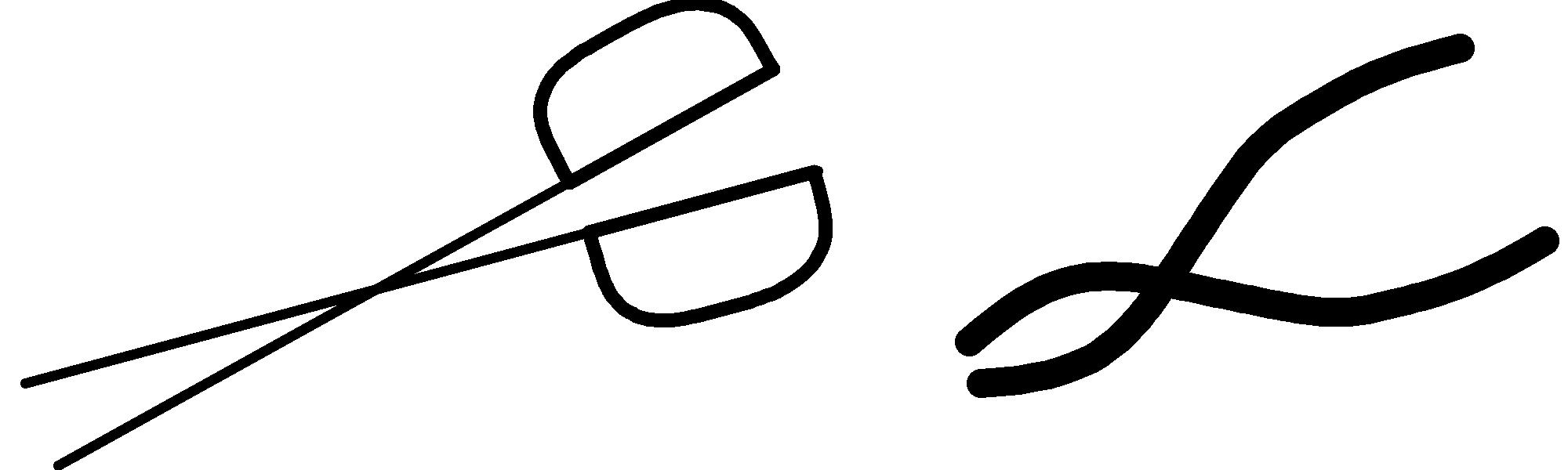
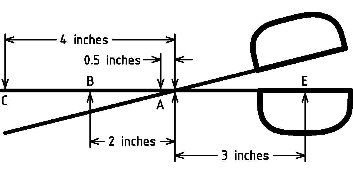
Suppose that you squeeze the handles of a typical scissors (shown below) together with 6 pounds of force applied at point E. What is the force applied at point A? At point B? At point C? [Hint: use exercise 3↑.]

4 The Wheel and Axle

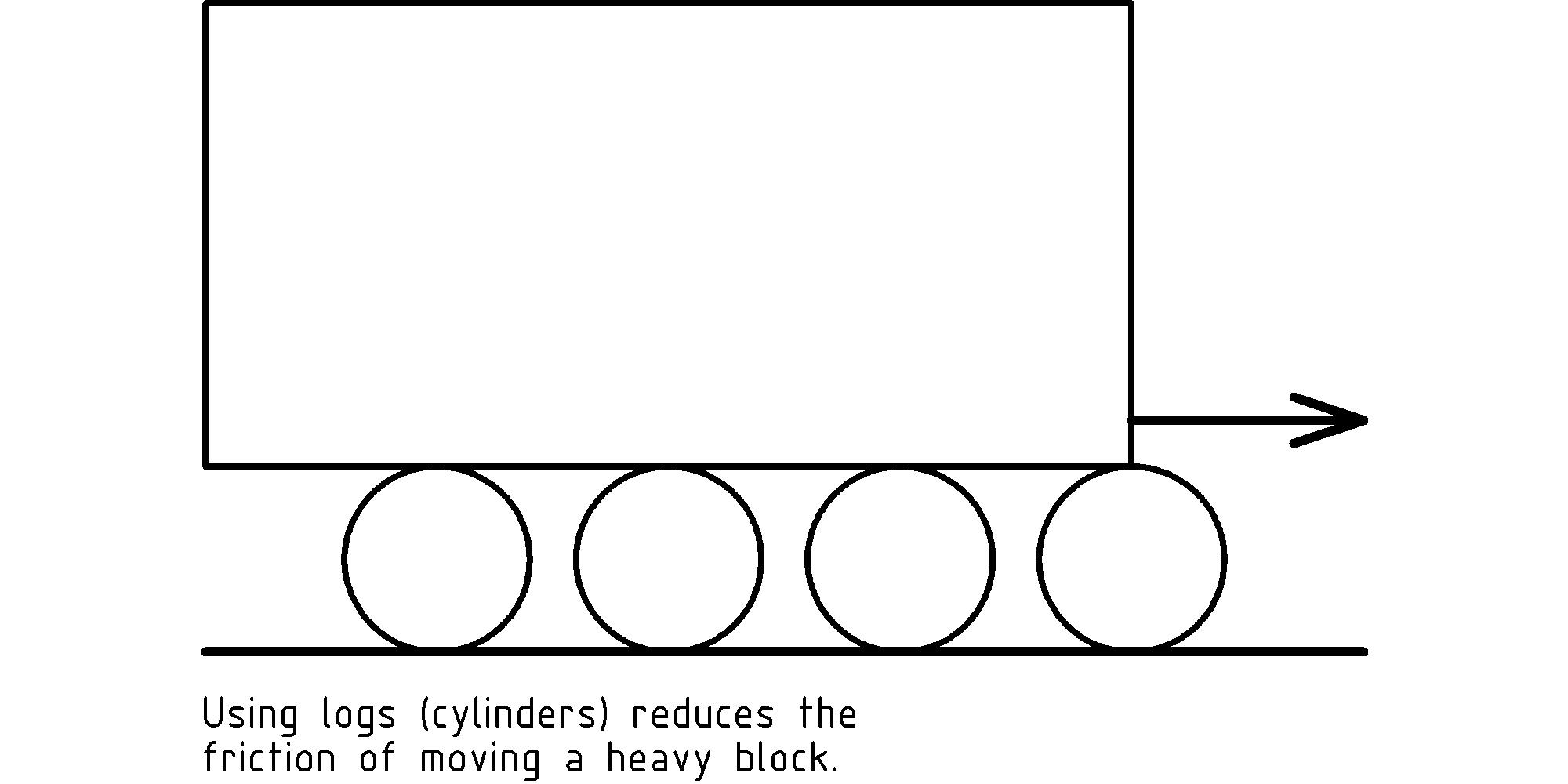
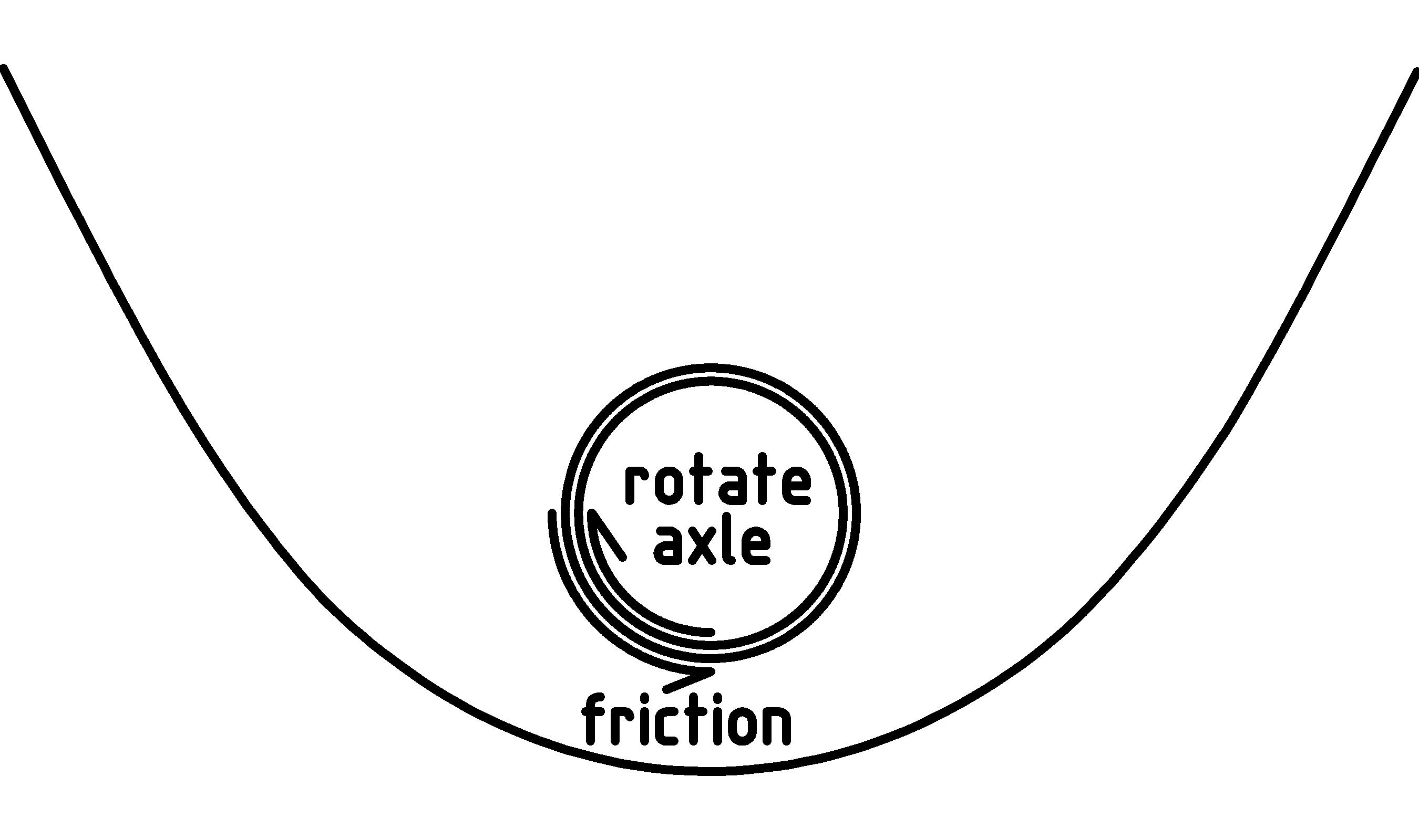
In this chapter we focus our attention on simple machines that bring the infinitely symmetrical shape of the circle to our aid in moving objects. To start, consider how a circular shape can be used to reduce the friction of moving objects much as ancient Egyptians are thought to have used logs to move the blocks of a pyramid:

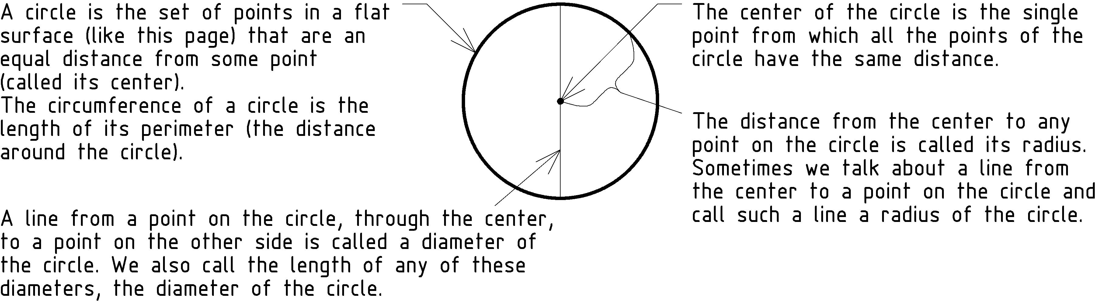
Before we take a closer look, let’s introduce some terminology:

Now consider what happens as we push the block to the right:

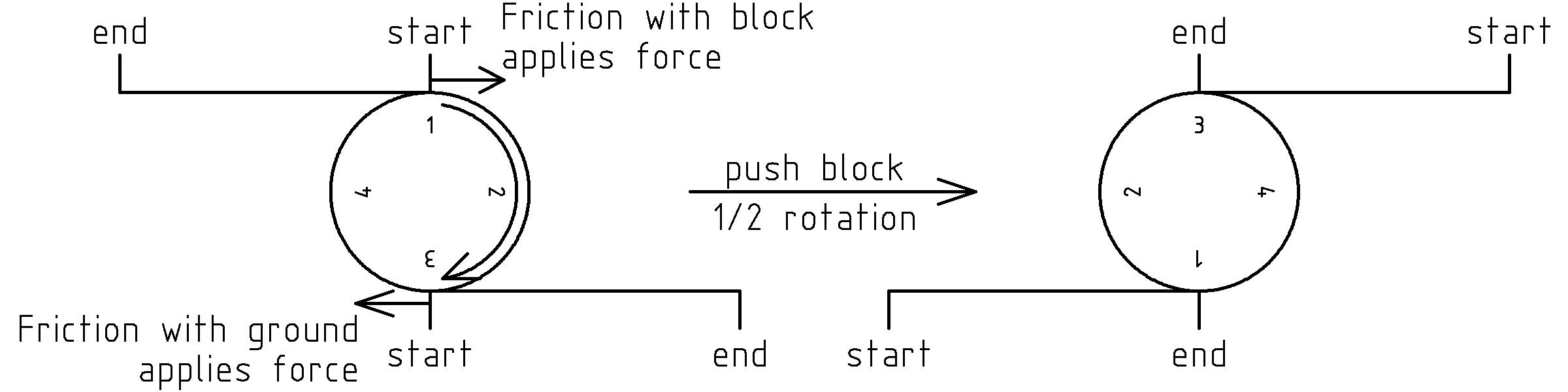
As we push the block, the friction between the top of the log and the block cause a resistive force (to the left) on the block. The top of the log feels this as a force (to the right) applied to the top of the log. Similarly, the friction between the log and the ground cause a resistive force (to the left) at the bottom of the log as the log is pushed to the right from the friction at the top. These forces on the top and bottom of the log in opposing directions cause it to rotate about its center, rolling along both the ground and the block.

We can reduce energy lost in friction by making the cylinders and their alignment perfect as well as making the block and ground more flat, smooth and hard. Suppose we reduce the friction so much that we can ignore it, and yet we still do a large amount of work in moving the block horizontally. Can you recall from chapter 2↑ where the energy is stored? In this case, the work is converted into the kinetic energy of the motion, not only of the block, but also the rotation of the logs.

However, even if we can keep everything properly aligned, one substantial problem with this configuration is that the cylinders will roll out from underneath the block: each half rotation causes the cylinder to move back on the block by one half of its circumference. In order to keep the circular shape (known as a wheel) in place and correctly oriented to help move objects, we attach each wheel to a shaft (known as an axle) that allows the wheel to be fixed in place and yet rotate as needed. This reintroduces friction with the rotation of the wheel, but keeps the wheels aligned, in place, and eliminates the need for the moving object to be flat.

We’ll soon look more closely at friction, but, first, let’s take a closer look at a simpler configuration of a wheel and axle ignoring friction for the moment.

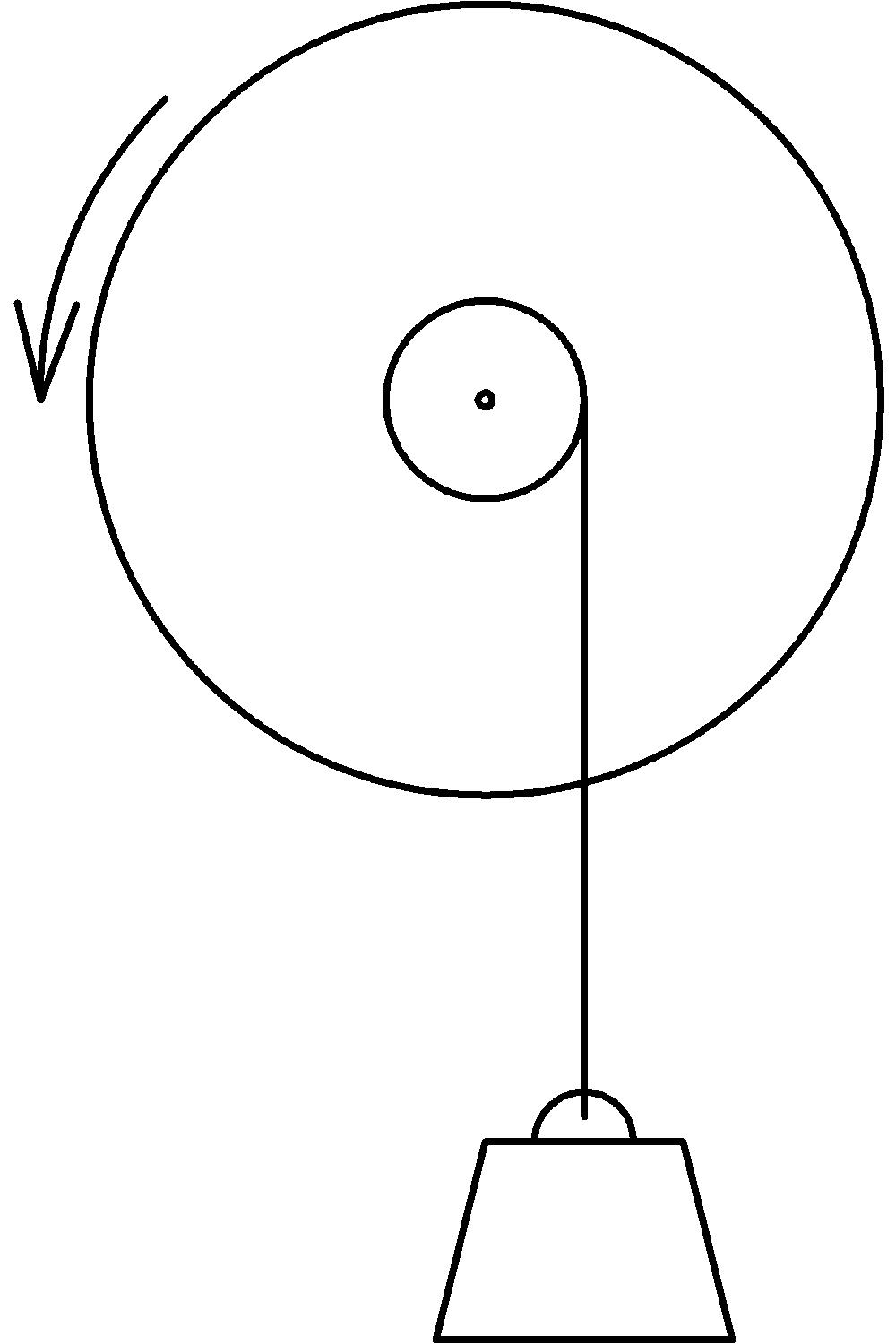
As we turn the wheel (we could use a belt or gear teeth around the circumference of the wheel, or just grab there with our hands to turn it), the line winds around the axle and lifts the weight. The question we’ll dig into further is: How does the wheel and axle help us lift the weight? To answer this, we’ll focus our attention on a slice of the configuration as follows:

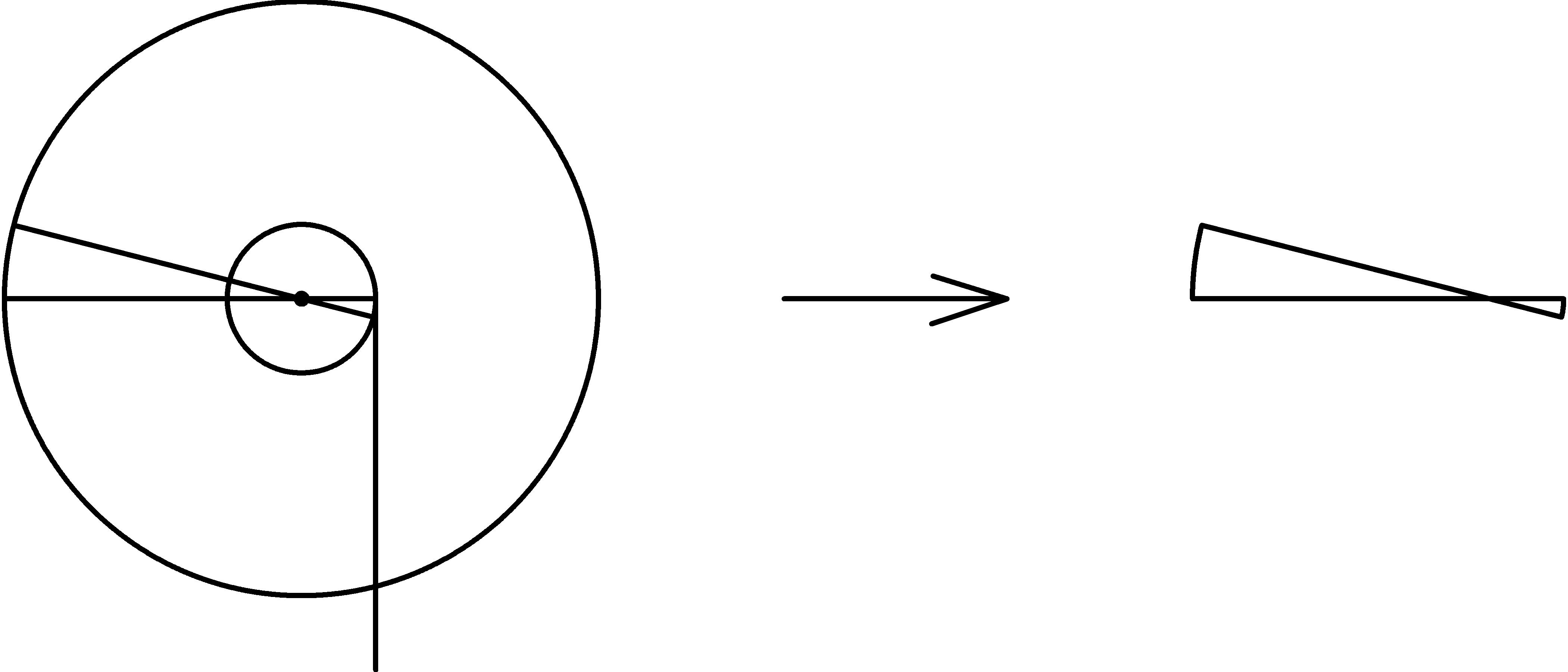
Hopefully, you’ll be able to recognize this as our lever diagram from page 1↑. In fact, a wheel and axle form a continuously rotating lever! In this configuration, the center of the axle (and wheel) is the fulcrum, each radius of the axle is a load arm, and each radius of the wheel is an effort arm.

From our earlier analysis of levers, we know that if the radius of the wheel is four times the radius of the axle, we will only have to use one quarter of the force required to lift the weight, but must apply that force through four times the distance (the circumference of the wheel as opposed to the circumference of the axle). In a similar way, if we can apply four times the force required to turn the axle, then the length of travel of a point on the outer edge of the wheel (around the circumference) will be four times as far as the motion of a point on the surface of the axle. It’s no wonder that vehicles with wheels can move so fast!

Now, let’s take a closer look at pushing a cart or wagon and see what happens with the axles attached to the cart:

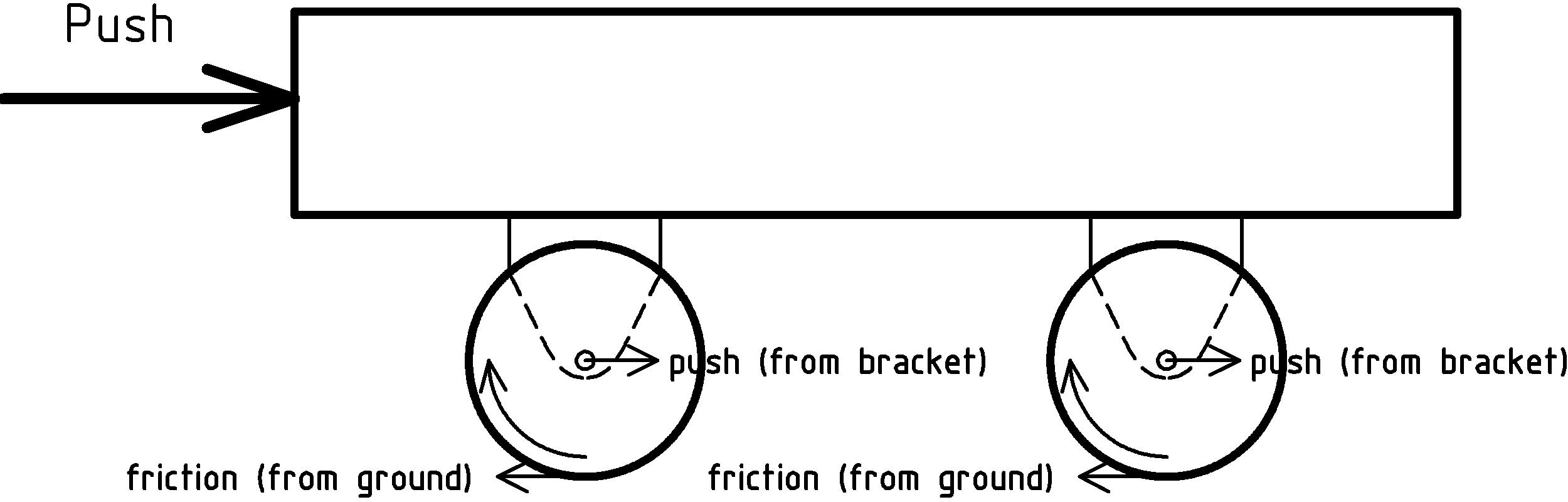
As we push the cart, it applies the force of our push to the axles through the attachment points. The friction between the wheels and the ground causes a resistive force to be applied to the wheels at the point where they touch the ground. The two opposing forces, one on the axle pushing forward, the other on the outer edge of the wheel pushing back cause the wheel to rotate.

The main difference between rotating logs under a block, and wheels and axles on a cart, is that the axles are held in place by a bracket, a bearing [N] [N] A bearing is an object whose purpose is to provide a surface to take on (without yielding) the force of contact of some other object., or some other material that will touch the axle as it rotates. This will introduce the resistive force of friction in a direction that opposes motion of the axle [O] [O] Rather than draw a bunch of little arrows all along the circumference of the axle, I just sort of joined them together into a bigger curved arrow. Most of the contact force and friction will occur on the top half of the axle.:

This concentrates the friction to the points of attachment for the axles. We can reduce the friction at these isolated places with various techniques that include making the surfaces smooth, hard, and slippery. Here is a device that, in addition, utilizes the freely rolling log idea, fixing balls around the axle with a special bracket that allows the balls to rotate almost freely:

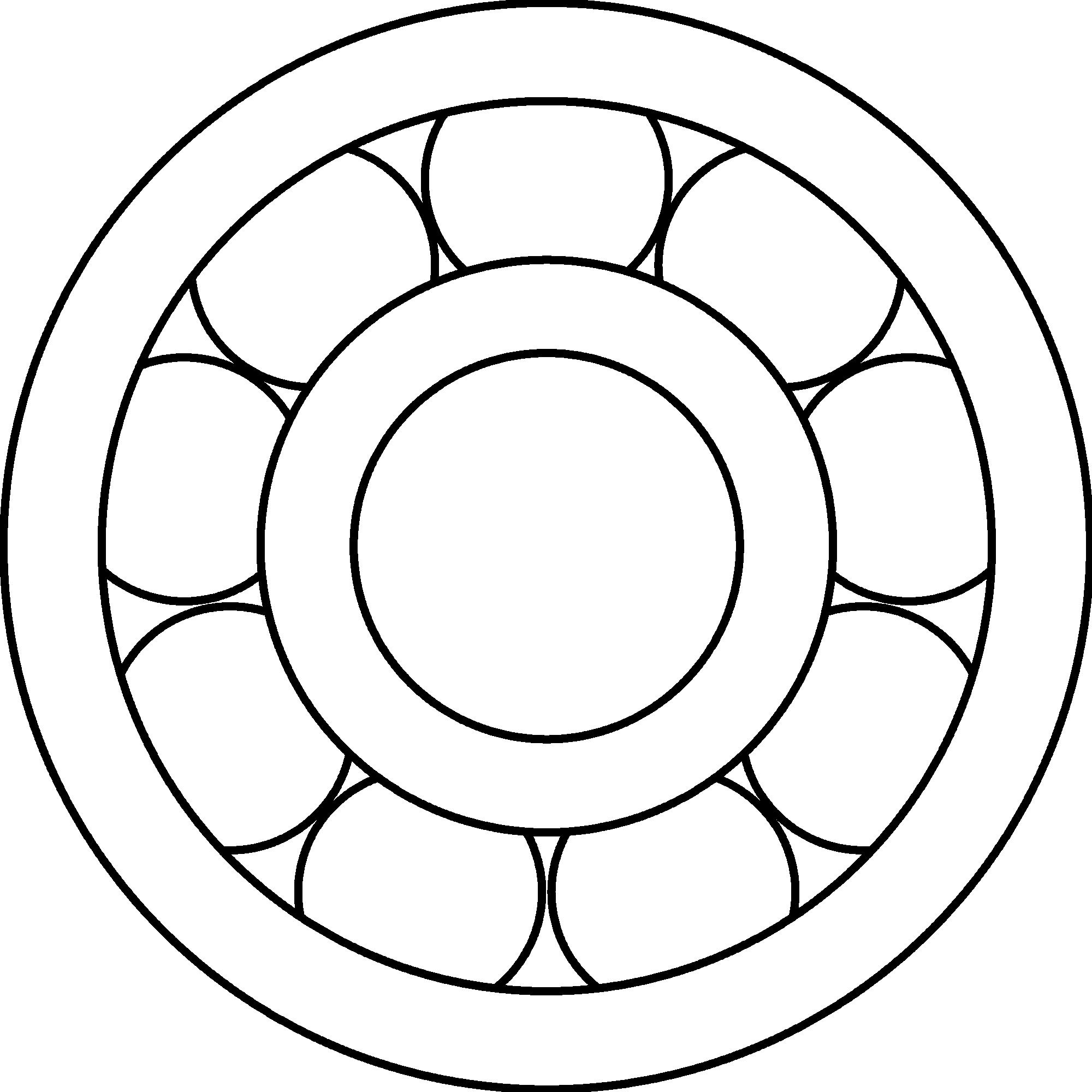
However, even without any special devices or attention to reducing friction (other than making sure the hole is big enough to let the axle to rotate freely), the rotating lever configuration makes the wheel and axle work. The multiplication of force due to a large wheel radius compared to a small axle radius can easily overwhelm a small frictional force resisting the rotation.

Before we end the chapter, let me mention that the continuous circular motion of the wheel and axle is so useful that it has spawned three different classes of simple machines. The first are rope and pulley systems that we’ll take a closer look at in the next chapter. The second are belt and pulley systems that link two rotating pulleys together using a flexible connector and friction. The third class locks rotating wheels (called gears) together with interlocking teeth.

Now, here are some exercises for you to check your understanding of the wheel and axle.

Exercises

Consider the block and log diagrams on pages 1↑ and 1↑. How many circumferences of a wheel does a block move when the wheel rotates two complete revolutions?
For this exercise [P] [P] Thanks to Leo Rice for this exercise. you need a couple of different sized wheels and some string.
1. Loop the string once around the circumference of the first wheel so that you have a length that represents the circumference of the wheel. Measure the circumference of the wheel by measuring the string.
2. Measure the diameter of the wheel (perhaps as its height when placed in a rolling position on a table).
3. Find the ratio between the circumference and the diameter of the wheel:
4. Repeat parts (a), (b), and (c) for the second wheel. Are the values similar?
5. What do you think would be the case for a third wheel with a different diameter?
Consider friction brakes for a bicycle wheel having a 32 inch diameter rim and a concentric (having the same center) 8 inch diameter disc.
1. All other things being equal, how much more effective are brakes on the rim of the wheel than brakes on the 8 inch diameter disk?
2. All other things being equal, how much more friction surface area must the disc brakes have to be as effective as the brakes on the rim?
3. What is another way of making the disc brakes more effective without changing either their distance from the center, or their friction surface area?

Suppose a water wheel, through the combination of kinetic energy of water falling into and the resulting weight of water in the buckets, can supply 50 pounds of force at a radius of 6 feet. Suppose further that the friction of the wheel is negligible.

Torque is a quantity, similar to work, that we define as the product of two terms: 1) the radius of the circle of rotation, and 2) the force at a point on the circle of rotation, in the direction of the circumference of the circle:
Torque = Force × Radius
What is the torque supplied by the water wheel in foot-pounds?

Suppose the water wheel is used to lift weights at various speeds by connecting the axle to different sized axles with ropes to lift them. Fill in the missing values in the following table for the maximum weight capable of being lifted by the water wheel using axles of the various specified sizes.

Max Load(A)/(A)	Radius	Torque
60 pounds(A)/(A)	30inches	30foot − pounds
300 pounds(A)/(A)
(A)/(A)	3 feet
(A)/(A)	1 foot
(A)/(A)	6 inches
(A)/(A)	3 inches
(A)/(A)	12 feet

5 Rope and Pulley Systems

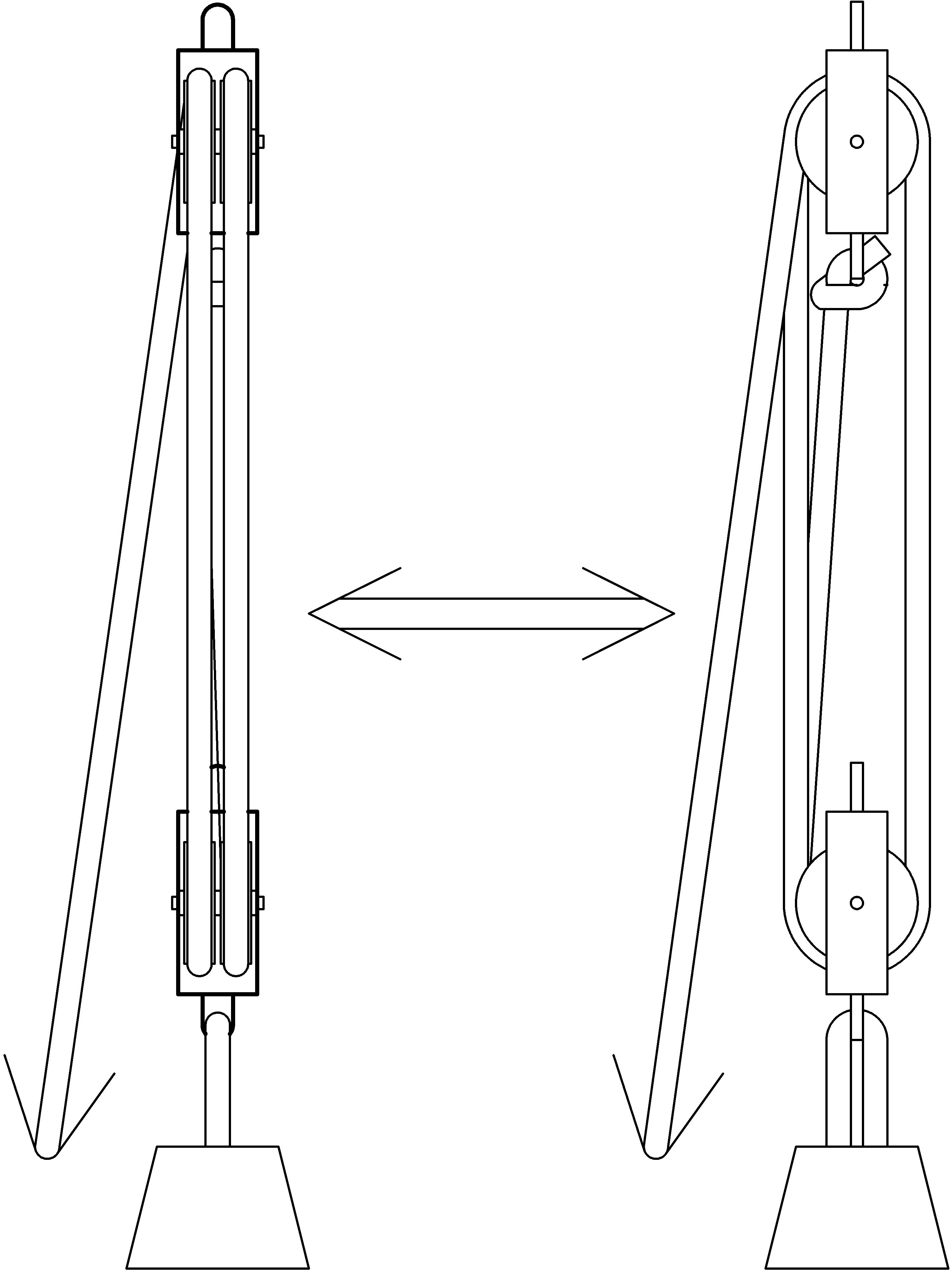
In this chapter we’ll take a look at a simple machine that is thought [Q] [Q] http://en.wikipedia.org/wiki/Block_and_tackle to be invented by Archimedes of Syracuse about 250 BC and is still in use, especially on ships with sails, even today. This simple machine is constructed out of a rope (or some similar strong, thin, flexible, but non-stretchable substance) and special wheels called pulleys that have grooves for the rope around their circumference. The groves on a pulley keep the rope from slipping off. One possible construction might look something like this:

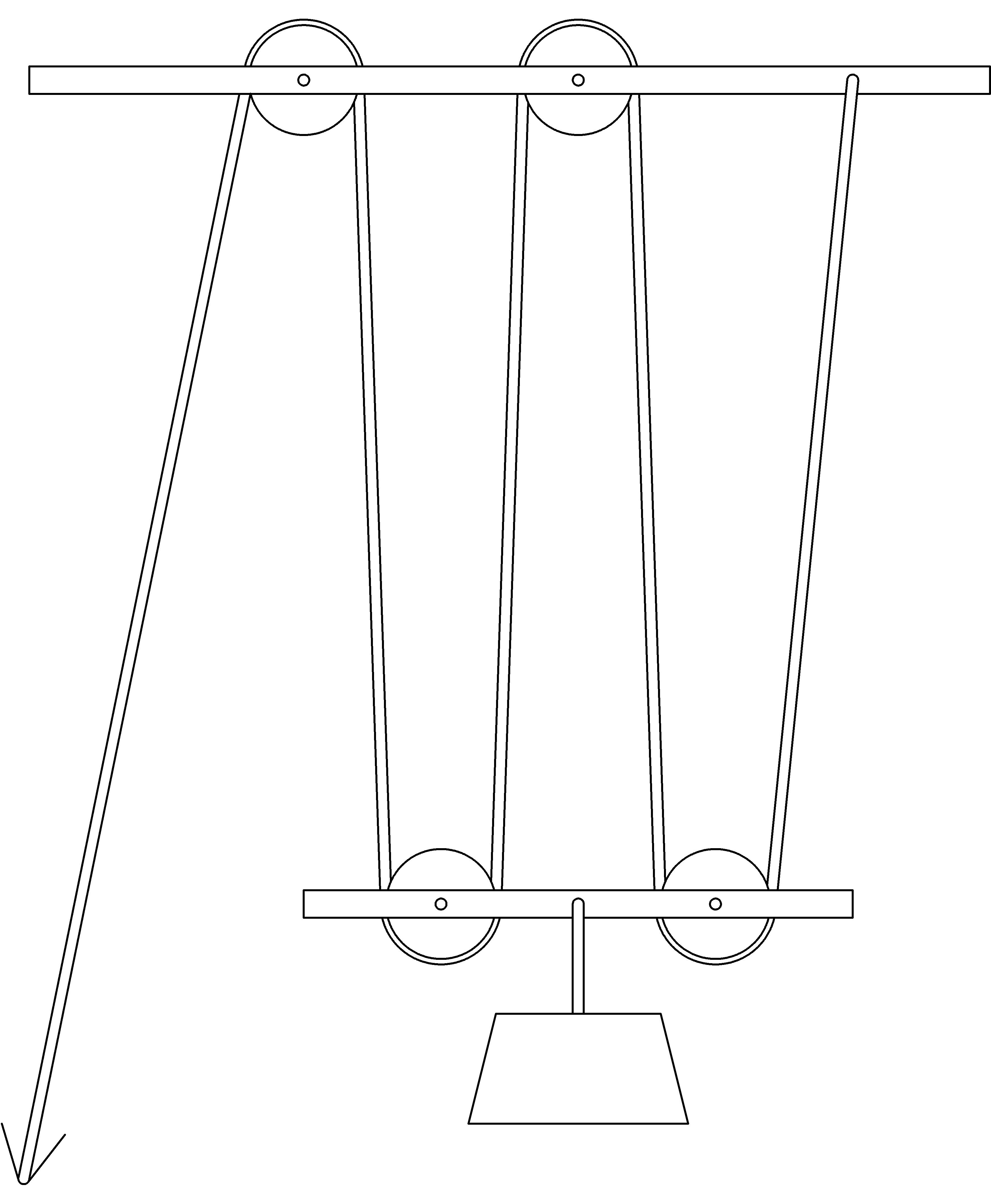
Notice the two groups of pulleys: one group attached to an overhead immovable object (such as an arch, ceiling rafter, or ship spar) and another group below, fastened together with a beam that is bearing some load to be lifted. The basic idea is to pull the rope in order to lift the object attached to the bottom set of pulleys. We arrange the system so that we pull down on the rope to lift the load, using our full body weight of force.

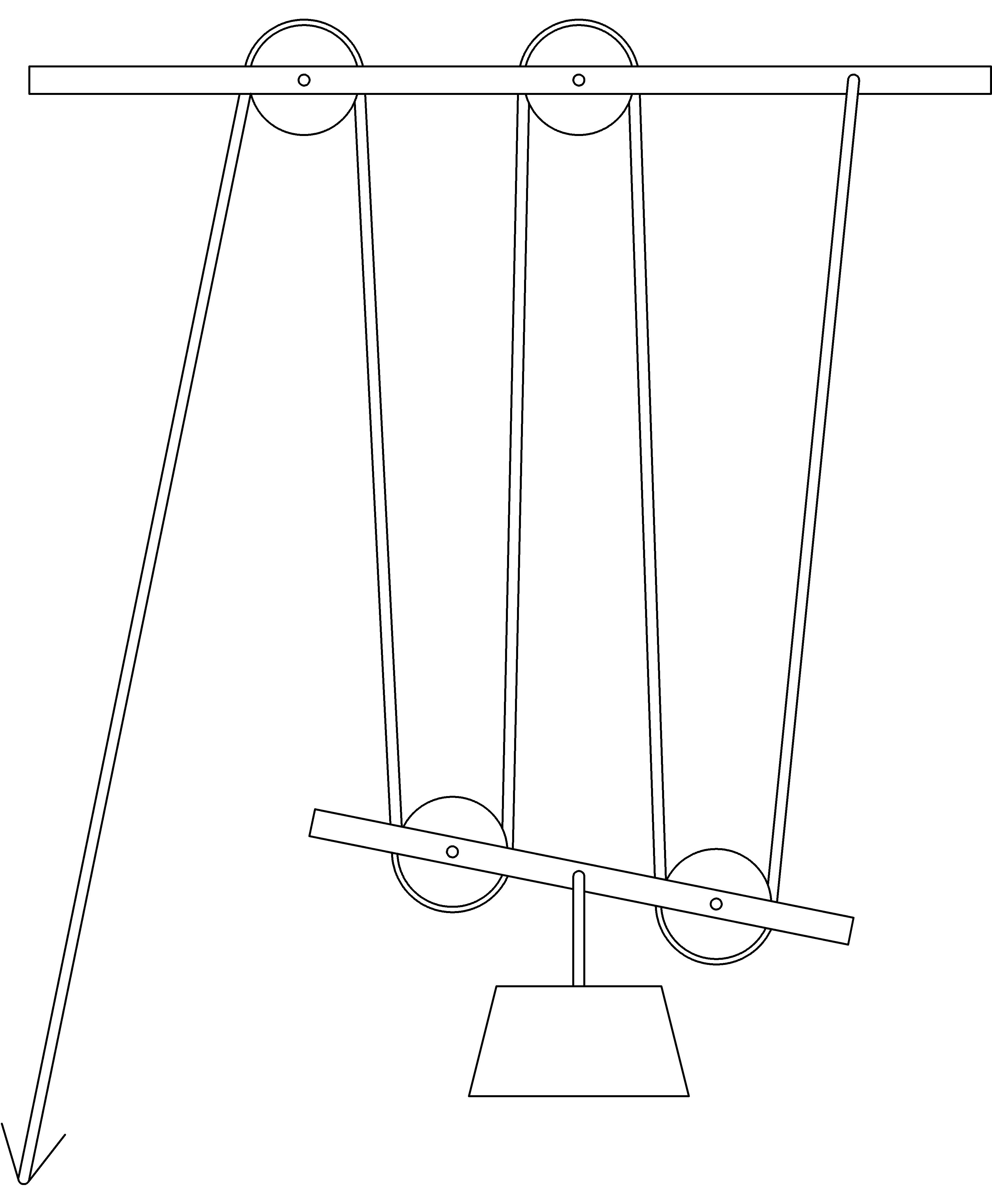
Before we can find out how much easier this rope and pulley system makes lifting things, we need to address a practical issue that hampers the proper operation of the construction shown above.

What we would like to have happen when we pull on the rope, is for the beam connecting the pulleys to move up, staying parallel to the ground. Can you guess what will really happen? Where does the rope first start to pull on the lower beam? Can you find the pulley that will first feel the lift from the rope? It is the one on the left. It will start to move up before the one on the right in a way that will minimize the lifting of the load:

Making the device as compact as possible eliminates this effect as well as making it easier to transport, attach, and fit into place. The pulleys are collapsed onto two axles, one at the top, and one at the bottom, yielding the arrangement given to us by Archimedes that we call a block and tackle shown below (the left view shows pulley edges, the right view shows pulley circumferences):

The block and tackle allows uniform lifting of the axle and uniform shortening of the rope segments connecting the upper pulleys to the lower pulleys. In order to more easily visualize and understand how this simple machine helps us work, we’ll use the first diagram where the pulleys are separated, even though in practice they’ll be configured into the block and tackle arrangement.

Let’s start by considering lifting a 24-pound object up one foot. We recall from chapter 2 the work equation:

Work = Force × Distance

If we plug in 24 pounds for Force and 1 foot for Distance we end up with 24 foot-pounds for the amount of Work. Now, let’s see how this works with a pair of pulleys above and a pair below:

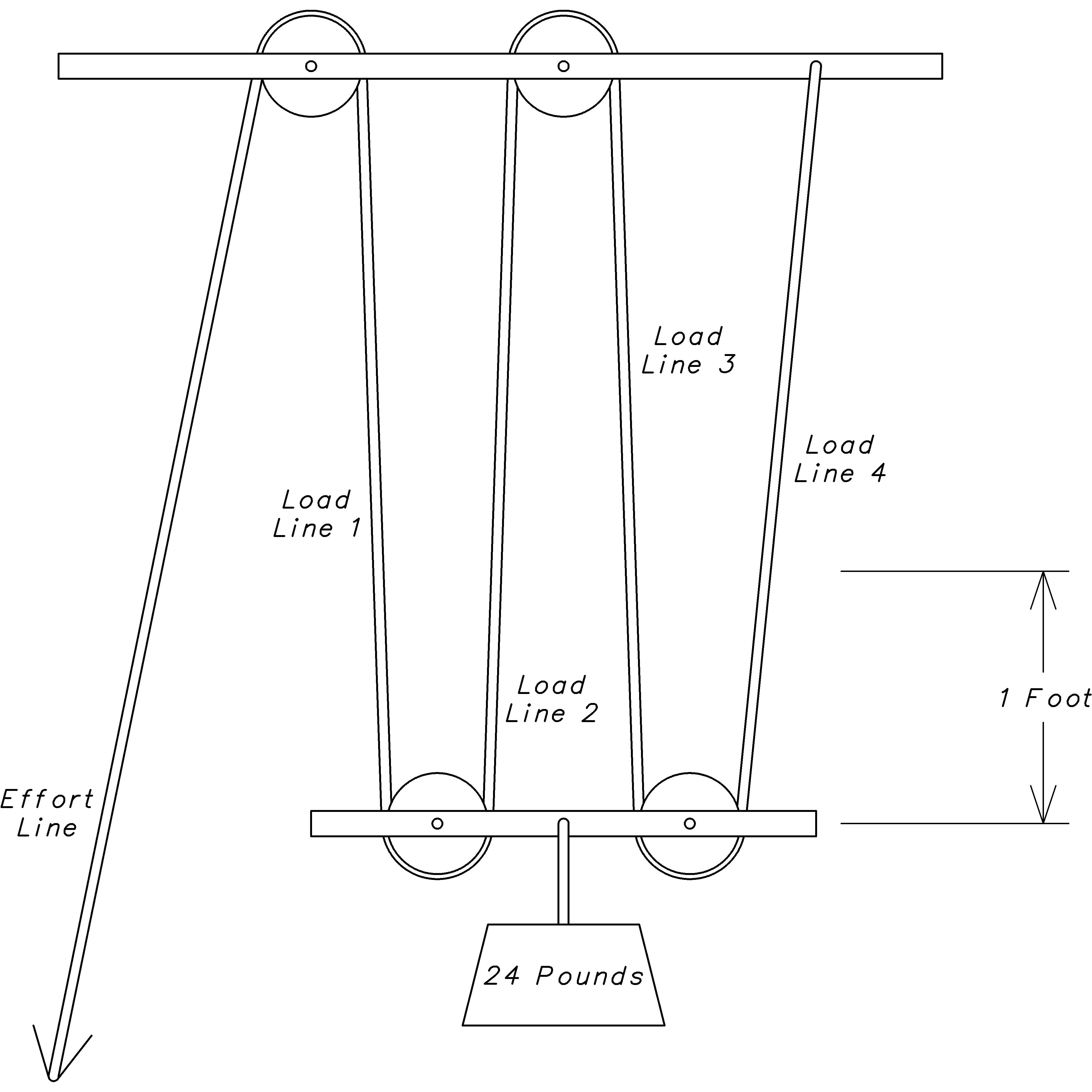
In keeping with the lever terminology, we’ll call the line that we pull the effort line, and the lines that run from pulley to pulley (or pulley to fixed attachment) load lines. In the case shown above, we have four load lines. Using this configuration to lift the 24 pound weight up 1 foot, we can see that all of the load lines must contract by approximately [R] [R] The more the upper pulleys are directly over the lower ones, as in a block and tackle, the closer to one foot the rope segments must move. one foot. This means that we must pull the effort line approximately 4 feet.

We now assume that the pulley and axle have minimal friction and invoke our work conservation principle to reason that the work of pulling the effort line is the same as the work of lifting the load. Lifting the 24 pound weight by 1 foot (ignoring the little friction in each pulley) is 24 foot-pounds. We also know the distance we must pull the effort line is 4 feet. Plugging these values into the work equation

24 foot − pounds = Force × 4 feet

we can see that the force required is only 6 pounds. In other words, the rope and pulley system reduced the force required to lift the object by a factor of 4. Furthermore, we can see that regardless of the object weight, the same reduction factor of 4 will apply, because there are exactly 4 load lines over which the effort is evenly spread, and this increases the distance over which the reduced force must be applied.

As with the other simple machines, we can see that when the work remains the same, the force reduction and distance magnification are linked as a consequence of the work equation:

Work = Force × Distance

When we keep Work constant and reduce Force by some factor, then Distance must increase by that same factor to keep Work constant.

This all assumes that we have ideal pulleys, that there is minimal friction between each pulley and its axle. Recall our discussion of friction for the wheel and axle in chapter 4↑. However, how would we have to modify the work equation if the friction becomes significant? For more on this try exercise 5↓.

Before you dig into the exercises, let me point out the advantage of using even just a single overhead pulley. Even though there is only one load line and one effort line, with this configuration you can more easily lift your body weight weight worth of load. Either grip the line and pull down with all your body weight, or tie a loop in the effort line a foot or two off the ground and stand in it. For an added twist, see exercise 5↓.

Exercises

Suppose you weigh 80 pounds, and you have a 4-load-line block and tackle attached to a sturdy beam in your garage. What is the most you can lift using only your own weight?
Draw a rope and pulley system with 2 load lines.
Draw a system with the most load lines using 3 pulleys.
Draw a pulley and rope system with 5 load lines.
Assuming downward effort, does a rope and pulley system with an even number of load lines anchor above or below?
How many pulleys are necessary for a system with n load lines?
Suppose you weigh 70 pounds, that you have a 4-load-line block and tackle attached to a sturdy beam in your garage. You need to lift a 320 pound object. How much weight do you have to put in your backpack to get the job done?
Suppose you don’t have any pulleys, but do have: a rope, the object you want to lift has a smooth, sturdy, axle-like handle, and there is a smooth, sturdy, axle-like bar overhead you can use to lift the object. Denote the weight of the object as F and the distance you need to lift it as d.
1. If you rig a 4-load-line block and tackle (without the pulleys, call each place you’d want a pulley a friction-point), how much weight will each friction-point feel?
2. Assume that the friction between the rope and axle is proportional to (say one tenth of) the weight felt. How much work is consumed by the friction at the friction-point closest to the rope anchor? The second closest? The third closest? The remaining one?
3. What is the total work consumed by all the friction points?
4. Give an expression using F, d, and the friction coefficient c = 1 ⁄ 10 for the total work required to lift the object.

A Simple Equations

Just as concise notes focus our attention and collapse a complicated subject into a comprehensible group of concepts, so do equations help us understand and reason about relationships. Think about how the work equation helps us understand the relationship between work, force, and distance. Embedded in the equation is not only our definition of work, but also the restriction: that to keep work constant, a reduction in force is necessarily accompanied by an increase in distance over which it is applied.

In this appendix we’ll follow in Archimedes’ footsteps and use the level in a purely abstract way to further our understanding of equations. Hopefully, this will help visualize what equations mean and how to work with them. Specifically, we’ll explore how a true equation is like a special kind of lever, a beam balance that is perfectly level (horizontal):

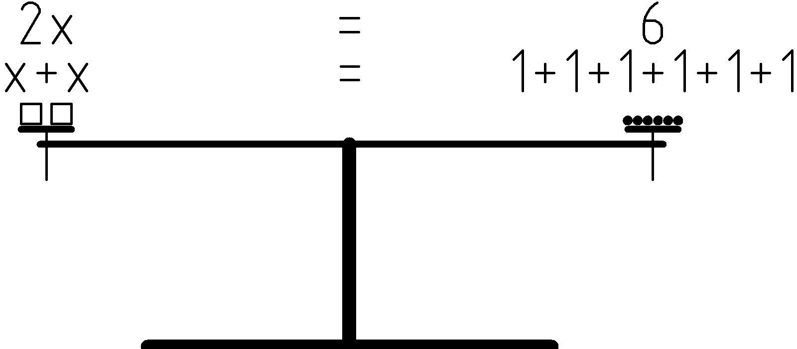
A beam balance has the left and right arm of the same length so that weights on each side are equal when the beam is horizontal or level. The horizontal or level position of the balance corresponds to truth of the equation. If the beam is horizontal, the weights are equal and the equation is true. The weight on the left hand side of the balance corresponds to the numeric value on the left hand side (LHS) of the equation, the weight on the right corresponds to the numeric value on the right hand side (RHS) of the equation. In the case shown above, the boxes on the left hand side represent the variable, or unknown quantity, x. The beads on the right hand side represent the integer 6.

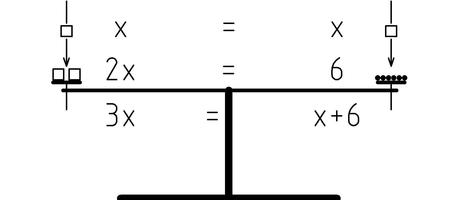
Let’s explore this a bit further. We could, for instance, add one box to each side and maintain the balance. This would correspond to the equation: 3x = x + 6. (In this appendix, I’ll often write products without using an explicit multiplication sign, or sometimes as a dot, to avoid confusion with the variable x.)

In principle we could add any number of boxes, say n of them, to each side and maintain the balance: 2x + nx = nx + 6. This corresponds to a principle that goes back more than 2000 years to Euclid. He captured it as Common Notion 2 in Book I of The Elements that can be translated as [S] [S] See Book I Common Notion 2 of Heath’s volume 1 of “Euclid: The Thirteen Books of the Elements.” The common notions are general principles used freely throughout the proofs (sequences of justifications for the truth) of the propositions.: “If equals be added to equals, the wholes are equal.”

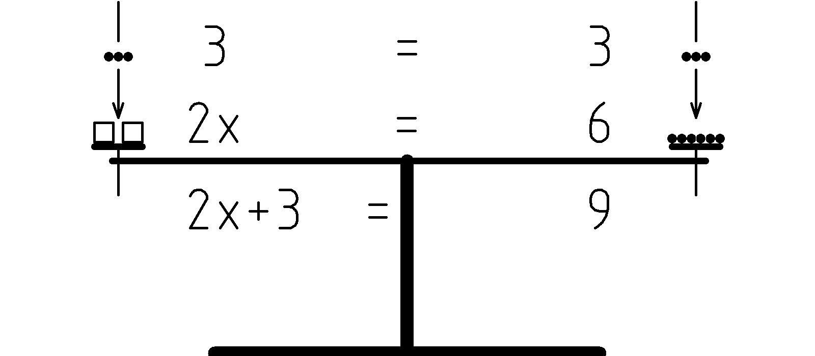
In a similar way, we could add equal numbers (beads), say 3, to each side to get: 2x + 3 = 9:

Or subtract equal amounts from each side to maintain the balance. Am I talking about the equation (x’s and numbers), the beam balance (boxes and beads), or both? Does it matter? Perhaps our analogy breaks down when we try to take away more than is present on the balance to end up with negative weight, but the principle still holds for an equation.

Alternatively, when starting from a balanced state, we should be able to double both the LHS and RHS and maintain the balance. This corresponds to the equation: 2(2x) = 2(6), which we can write as: 4x = 12:

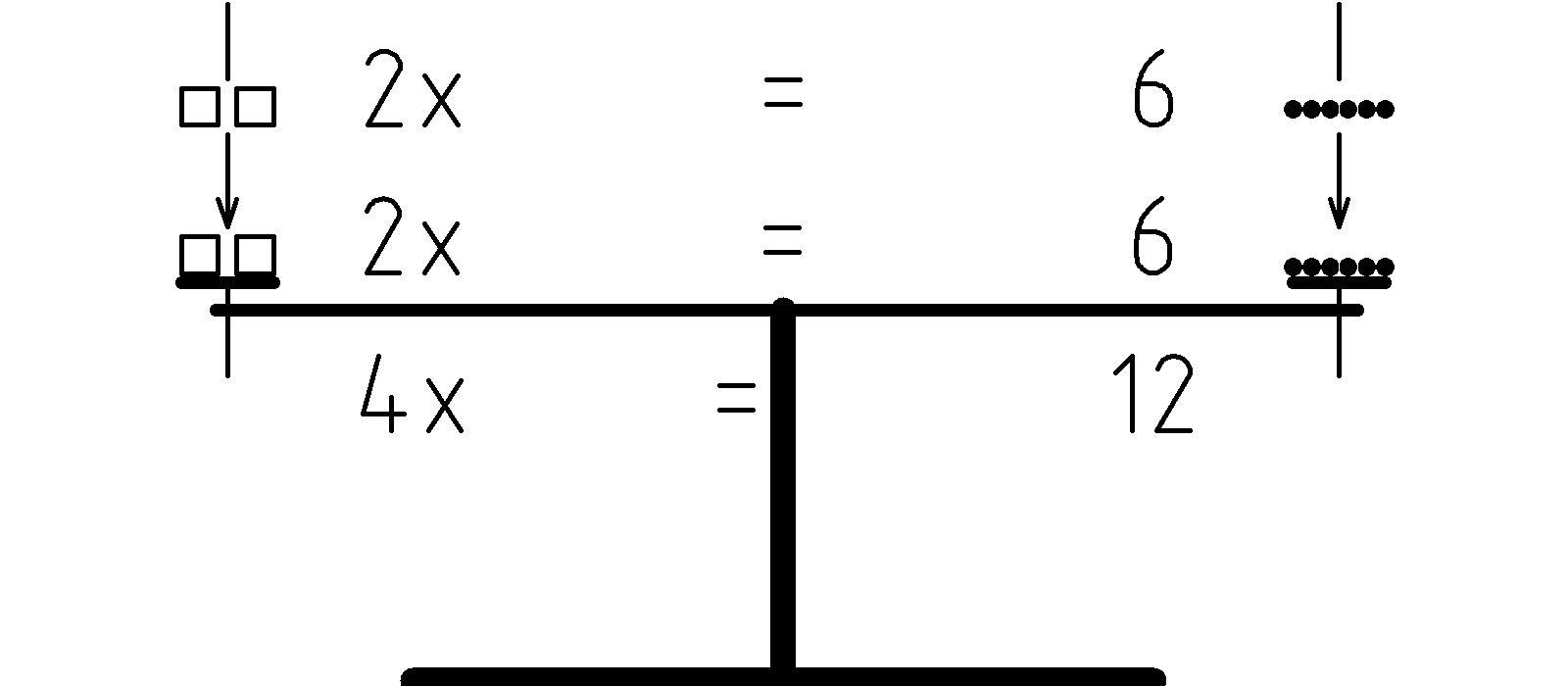
However, in principle, we could triple, quadruple, or, more generally, multiply by n both the LHS and RHS and maintain the balance: n(2x) = n6.

Similarly, we can divide each side in half, leaving one half on each side and maintain the balance. This corresponds to the equation: x = 3. Hopefully, you can begin to see how useful these operations are for solving simple equations.

Once again our analogy causes some difficulty when generalizing division of both sides by any number, where in the case of the balance we think in terms of whole objects, but again it remains true for equations: 2x ⁄ n = 6 ⁄ n as long as n is not zero.

We can even combine the multiplication (by n) and division (by non-zero d) into multiplication on both sides by one number, the fraction n ⁄ d:

(n)/(d)(2x) = (n)/(d)6

Let’s summarize all these operations that maintain the truth of an equation with the following symbolic rules by saying that if we have some equation:

LHS = RHS for example 2x = 6

then for any number c, whether it is positive, negative, integer, fractional, or decimal (including decimal numbers that cannot be written as fractions), the following are also true: LHS + c = RHS + c for example 2x + 4 = 6 + 4 LHS − c = RHS − c 2x − 6 = 6 − 6 c(LHS) = c(RHS) 5(2x) = 5⋅6
and for non-zero c:

(LHS)/(c) = (RHS)/(c) for example (2x)/(2) = (6)/(2)

Example 1: A Word Problem

Our first example goes like this: “Kate is two years older than her sister Madeline and three years older than her brother Doug. All together, their ages add up to 49. How old is Kate?”

To begin, we need to write this down symbolically. We’ll choose our variable x to be Kate’s age in years. Then Madeline’s age will be x-2 and Doug’s age will be x-3. We can write down the information given to us in the following equation:

x + (x − 2) + (x − 3) = 49

We’ll start by collecting the variables on the LHS, as well as the numbers. We have three x’s altogether, and we are taking away five altogether, so we have:

3x − 5 = 49

Our general strategy will be to perform operations on the equation until we end up with x all by itself on the LHS giving us the answer. Our next step will be to add 5 to each side of the equation, and then we’ll dived both sides by 3 to get the answer:

3x − 5 = 49 3x = 54 x = 18

Finally, we’ll check our answer by substituting the values back into our original equation:

18 + 16 + 15 = ? = 49

Example 2: Area of Triangles

Let’s examine the area of triangles using what we know about rectangles. We’ll start by recalling that the area of an 8 by 4 rectangle is 8⋅4 = 32 squares (units of area):

In a similar way, any rectangle with sides having whole-number lengths n and m will have the area: nm (remember, this means n times m). We can extend this same area rule to rectangles with sides of any positive lengths b and h using the same expression: bh. Let’s write this as the equation: area_□ = bh.

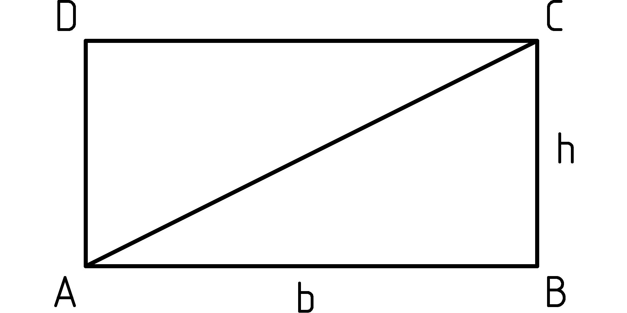
Now if we can agree that drawing a diagonal across a rectangle splits it into two equal [T] [T] In modern language, we say they are congruent. Euclid Book I proposition 4 tells us these triangles are equal since: 1) line segment AB is congruent to CD, 2) BC is congruent to DA, and 3) angle ABC is the same square angle as CDA. See Heath’s “Euclid: The Thirteen Books of The Elements.” This is commonly known as the SAS rule, and even though Euclid includes it as a proposition with an argument for its truth, it really is a postulate or axiom, something that we simply accept as true. triangles, then we we’ll have the area of the rectangle being twice the area of the triangle:

area_□ = 2 area_△

However, we also know that the area of the rectangle is: bh. We now use a principle whose truth is beyond question in both algebra and geometry, Euclid’s [U] [U] See Book I Common Notion 1 of Heath’s volume 1 of “Euclid: The Thirteen Books of The Elements.” Common Notion 1: Things which are equal to the same thing are also equal to one another. This means that we can substitute the product bh in place of the area of the rectangle area_□:

bh = 2 area_△

We can now divide both sides of this equation by 2 (that’s the same as multiplying by 1 ⁄ 2) to find the area of a triangle with a square corner at the base, base length b, and height h at the square corner as:

area_△ = (1)/(2)bh

Square corners are special in geometry. Euclid [V] [V] See Book I Definition 10 and Postulate 4 of Heath’s volume 1 of “Euclid: The Thirteen Books of The Elements.” called them right angles, defined so that adding two of them makes a straight line, and assumed each right angle is equal to any other. We call a triangle that has a right angle as a corner a right triangle, and just as a right angle is special, so is a right triangle.

So, how do we find the area of a triangle that doesn’t have a square corner? Just as we used rectangular area to figure out the area of a right triangle, we’ll use what we know (area of a right triangle) to figure out what we don’t (area of a triangle without a square corner at the base). Let’s start with the case of a triangle with the peak over the base. We’ll just draw a vertical line down from the peak to the base to end up with two right triangles:

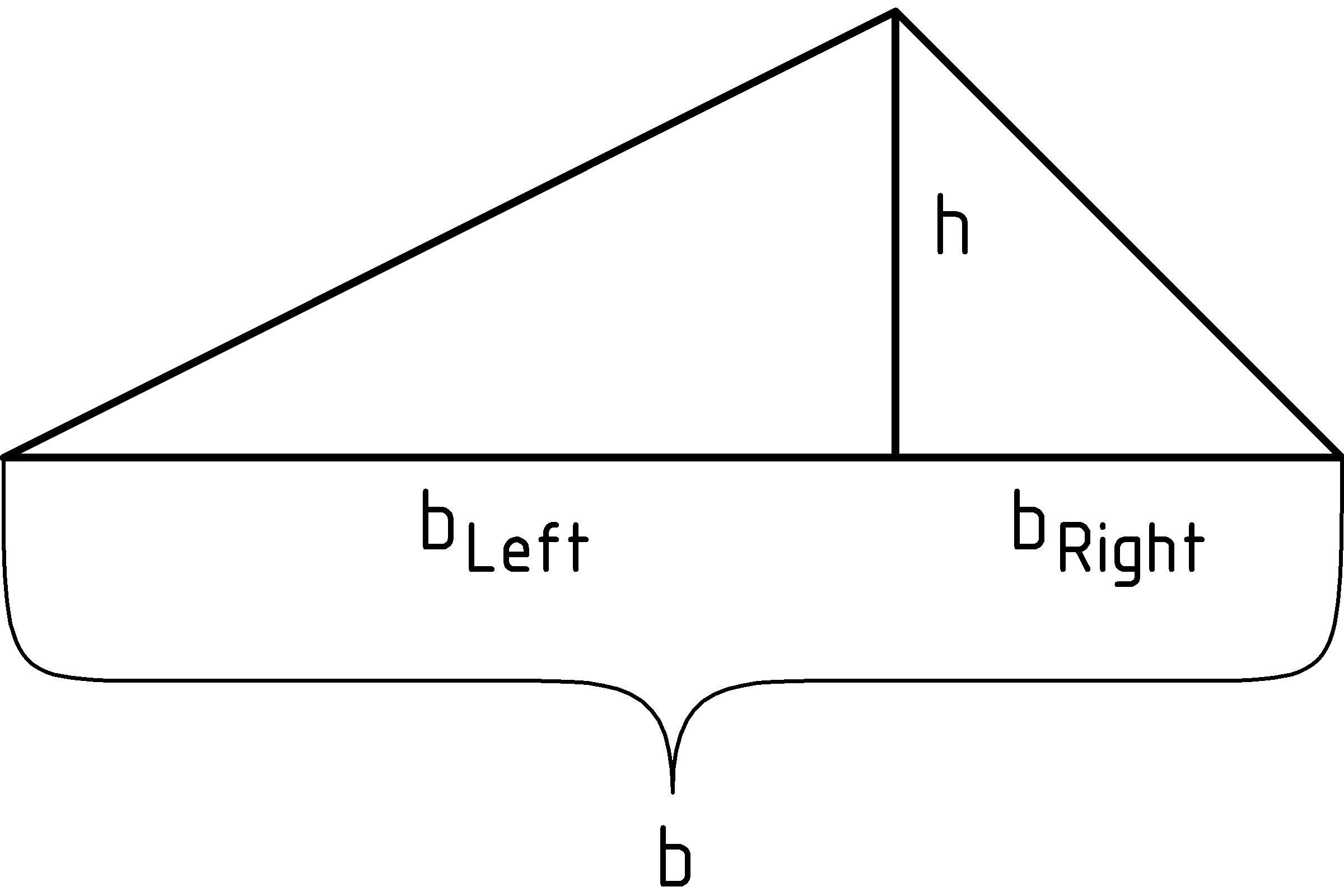
First we’ll express the area of the original triangle as the sum of the area for two right triangles, then we’ll substitute the expressions for these (since we know how to calculate them), and then we’ll regroup:

area_△ = area_L + area_R = (1)/(2)b_Lh + (1)/(2)b_Rh = (1)/(2)(b_Lh + b_Rh) = (1)/(2)(b_L + b_R)h = (1)/(2)bh

We can factor out 1/2 and h and group the addition of b_L + b_R for the same reasons that 7⋅10 + 7⋅3 = 7⋅13.

For the remaining case of a triangle with the peak not over the base, let’s still draw a line down vertically to the point where it meets the extension of the triangle base.

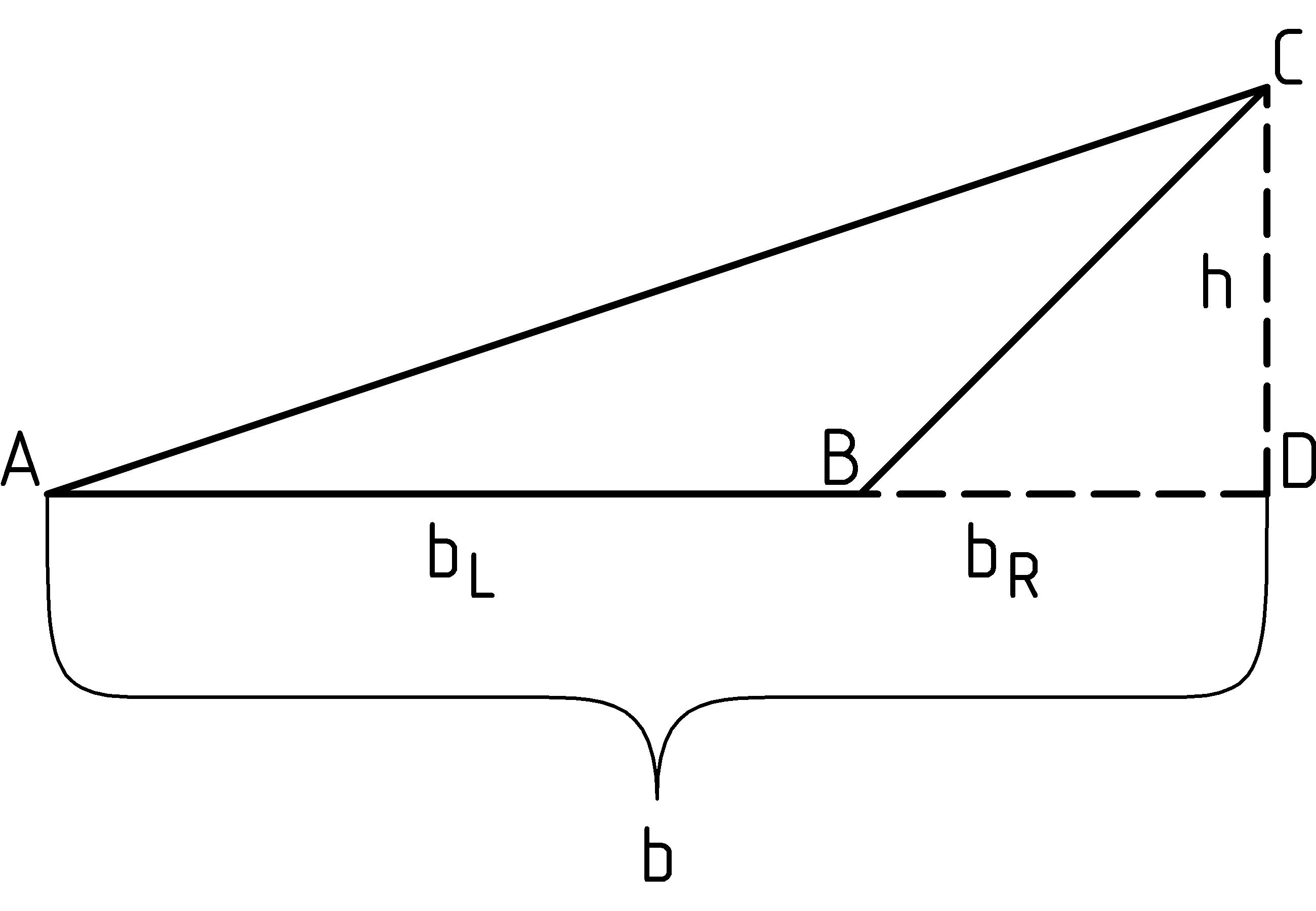
For our calculation this time, we’ll calculate the area of triangle ABC as the area of triangle ADC minus the area of triangle BDC:

area_{△ ABC} = area_{△ ADC} − area_{△ BDC} = (1)/(2)bh − (1)/(2)b_Rh = (1)/(2)(bh − b_Rh) = (1)/(2)(b − b_R)h = (1)/(2)b_Lh

We begin by first substituting the expressions for the area of the right triangles. The next steps are to again factor out both 1 ⁄ 2 and h and group the subtraction of b_R from b. Again, we can do this for the same reasons that 5⋅20 − 5⋅2 = 5⋅18. Next, since b − b_R is just b_L, we substitute b_L for b − b_R to get our result.

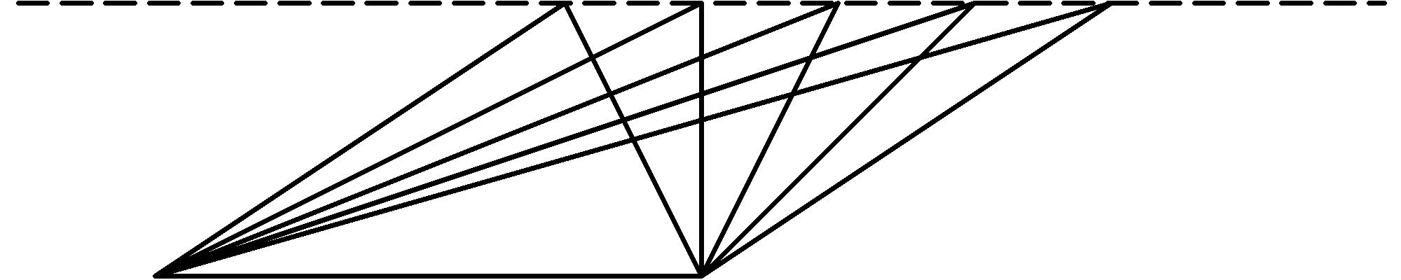
We have found that, just as for right triangles, each triangle without a right angle (peak over the base, peak outside base), the area is also one half of the base times the height. This also helps us understand the meaning of the height of a triangle. It is the distance that the peak of the triangle rises above the base along a square corner (or right angle). In the diagram below, the 5 triangles are all on the same base and have the same height (peaks on the dotted line) and so have equal areas [W] [W] Heath’s translation of Euclid’s proposition 37 of Book I is: Triangles which are on the same base and in the same parallels are equal to one another. Our intuitive approach to understanding this result is algebraic whereas the beauty of Euclid’s approach is in the self-contained system of Euclidean Geometry that derives results from definitions, postulates, common notions, and previously obtained results using deductive reasoning, a system that has been a successful model for mathematics and formal reasoning for 2300 years. :

Now, try your hand at the following exercises to practice and check that you can work with equations. If you are not sure of your answer, don’t let it go, be sure to check with someone who will know and can help you understand it.

Exercises

See also exercises 1 and 2 on page 23 of Chapter 3.

Solve the following equations for x (and check your answers):
1. x + 3 = 15
2. x ⁄ 4 = 12
3. x ⁄ 4 + 3 = 15
4. 2x − 3 = 17
5. x − 7 = 3x − 19
Kate is two years older than her sister Madeline and four years older than her brother Doug. All together, their ages add up to twice Kate’s. How old is Kate?
This exercise explores an equations for scale models. Suppose that you know the dimensions of an object such as a bridge (perhaps from architectural drawings), and want to make a model of it that is smaller, so that each piece of the model is smaller than in the real bridge by the same factor. Let’s use the following equation where the size of a piece r in the real bridge is multiplied by the scale factor f to give the size of the piece m in the model:
r⋅f = m
1. Suppose that the real bridge is 500 meters long, and that you want to build the model so that it is exactly 1 meter long. Substitute the numbers into the scaling equation and solve for the scale factor f.
2. Find out how big a model support should be if that support is 25 meters long in the real bridge, by substituting the scale factor you found in part (a) into the scaling equation for f, substituting the real length 25 meters in for r, and solving for m.
3. Convert the size of the model piece your found in part (b) from meters to centimeters by multiplying it by 100.
This exercise asks you to convert the lever-work equation of Chapter 3↑ page 1↑:
Load⋅Work_Distance = Effort⋅Effort_Distance
into a (perhaps) more usable form by using the scaling equations:
Work_Distance⋅Scale_Factor = Effort_Distance Load_Arm⋅Scale_Factor = Effort_Arm
1. First, divide the “distance” scaling equation by Work_Distance to find the first expression for the Scale_Factor.
2. Second, divide the “arm” scaling equation by Load_Arm to find the second expression for the Scale_Factor.
3. Next, divide both sides of the lever-work equation by Work_Distance and group the distance terms into a fraction on right hand side.
4. Now, recognize the fraction on the right hand side of the equation you get in (c) as the first expression for the Scale_Factor you found in part(a), and substitute in its place the second expression for the Scale_Factor you found in part (b).
5. Finally, multiply the equation you find in part (d) by Load_Arm to end up with the following leverage equation :
  Load⋅Load_Arm = Effort⋅Effort_Arm
6. Suppose you have a 20 pound bag of grass seed, placed on a teeter-totter 6 feet from the pivot point, and that you balance the teeter-totter when you stand 1 and 1/4 feet from the pivot point. How much do you weigh?

B Vectors

In this appendix, we examine more thoroughly the algebra of vectors, including how adding vectors in a line reduces to the algebra of numbers (scalars). Our final stop will be the full vector algebra formulation of the work equation.

We’ve already talked in chapter 1↑ on page 1↑ about how forces have both a magnitude (amount of push or pull) and a direction. How they are conveniently represented by arrows, and how these arrows form an algebraic system of what are known in mathematics and physics as vectors. Sometimes, instead of arrows, people refer to the representations as directed line segments. In this appendix, we’ll take a closer look at this algebraic system of vectors, starting with a different example, one that may seem more natural than forces.

You’ve already had a couple of hints about this more familiar system of vectors. In fact, you may already have guessed what it is. Recall from chapter 1↑ when we were talking about two forces canceling each other out and adding up to zero. Now think about the part of chapter 2↑, lifting a stone twice as far, which might suggest adding the lift distances. What am I talking about? I am talking about straight-line displacements: a motion, or movement, some distance along a straight line. We can even dispense with the “straight line” restriction if we are willing to consider only the start and end points of the motion (though, in more complicated cases, the intermediate path can make a difference).

Each displacement can be represented as a combination of magnitude or size (the distance from the start to end point) and a direction (from the start point to the end point). This combination of magnitude and direction of displacements can be represented by an arrow with the tail at the start point and the tip at the end point.

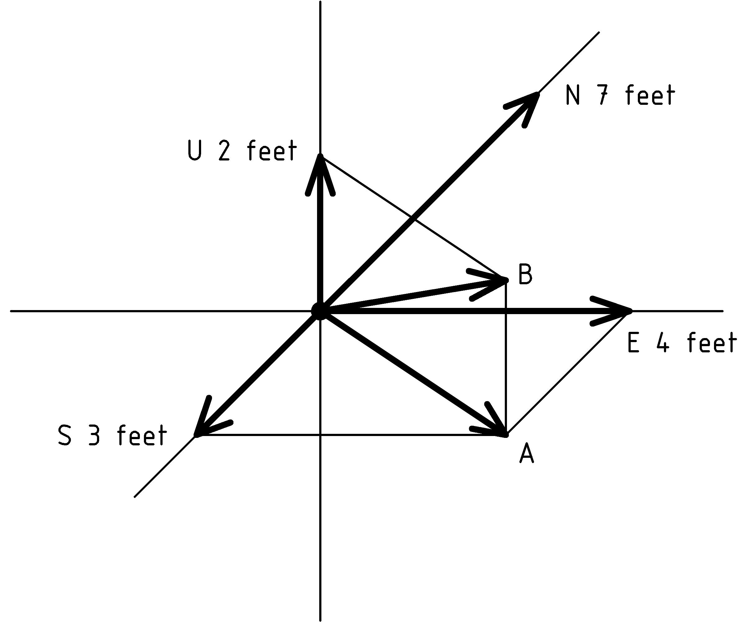
There are six vectors represented in the diagram above. Four of them are labeled with their direction [X] [X] Let’s use the first letter of the directions : Up, Down, North, South, East, and West. and length and the remaining 2 vectors are labeled A and B. The diagram is meant to depict three dimensional objects. To understand the diagram, we imagine that north is straight ahead into the page, so the displacement vector N 7 feet is 7 feet into the page (in the direction of the page in front of us). We imagine the vector S 3 feet points out of the page (from the page towards us) 3 feet, the vectors A and B point out of the page to our right, and the vectors U 2 feet and E 4 feet lie in the plane of the page.

With displacements as our intuitive guide to vectors, let’s dive right in and talk about algebraic operations involving vectors, starting with scaling.

Scaling Vectors

The concept of scaling an object is, essentially, to change its size with all parts either growing or shrinking by the same amount so that the shape stays the same. We associate this concept with the mathematical operation of multiplication by a number called the scale factor, or scalar, that represents this shrinking or growing amount. For example, consider making the displacement vector S 3 feet twice as long. This would become a displacement of S 6 feet. We can write this as:

2( S 3 feet) = S 6 feet

In a similar way we could scale the vector A by a (scale) factor of 2 writing the result as: 2 A. Or we could make it half as long via any one of: 1 ⁄ 2 A, 0.5 A, or A ⁄ 2. Moreover, we can scale any of the vectors, say B, by any scalar c as: cB. Notice that scaling a vector changes its length, but not its direction (depending on how you think about opposite directions). Let’s take a closer look at this by focusing on the NS line, ignoring measurement units like feet or meters for the time being, with the vector N 1 pointing to the right:

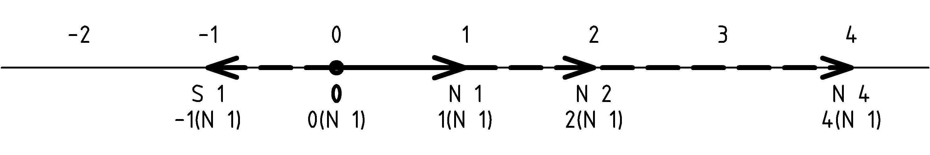
Notice that scaling by 2 gives N 2, scaling by 4 gives N 4, and scaling by 0 gives a vector with 0 length. Notice that this last vector has no length. In this sense it also has no direction. On the other hand, it can have any direction we care to choose, and since there is no length, it doesn’t really matter. For these reasons, let’s denote this zero vector using just its length, 0. To distinguish the zero vector from a scalar (we haven’t defined multiplication of two vectors yet, and when we do, it will be different from scaling), we’ll denote the zero vector in boldface as: 0.

Now, this last scaling result will be true for any of our force or displacement vectors. Scaling any of these vectors, V, by zero will give the zero vector:

0 V = 0

Next, notice that scaling N 1 by 2 gives N 2, and that scaling N 2 by 2 gives N 4. We can write this as: 2(2( N 1)) = 2( N 2) = N 4 = 4( N 1). This is another result that will hold for any of the force and displacement vectors, V, and any scalars a and b:

a(b(V)) = (ab)V

What about scaling by negative numbers? If we think of multiplying by a negative number as giving a scaled vector in the opposite direction, changing a north vector into a south vector, then we will keep the scaled vectors on the line so that integer multiples of N 1 correspond to integers on the number line. In terms of our vectors, we’ll have: − 1( N 1) = S 1. In a similar way, we can think of multiplying the vector S 1 by negative 1 giving the vector in the opposite direction: − 1( S 1) = N 1.

This gives us a geometric interpretation of multiplying by minus one as changing to the opposite direction. Combining these last two equations we have: − 1( − 1( N 1)) = − 1( S 1) = N 1 = 1( N 1). This lets us interpret the equation − 1 × − 1 = 1 as: changing to the opposite direction twice is the same as not changing at all.

We’ll soon see that this interpretation will continue to make sense when adding vectors, which is our next topic.

Adding Vectors

The rule for adding vectors is essentially the same as combining displacements when you think about it in the following manner. To help us visualize, let’s be specific and consider the displacements N 3 feet and E 4 feet. How should we combine these two displacements? Hopefully, it will seem natural to move north 3 feet and then move east 4 feet:

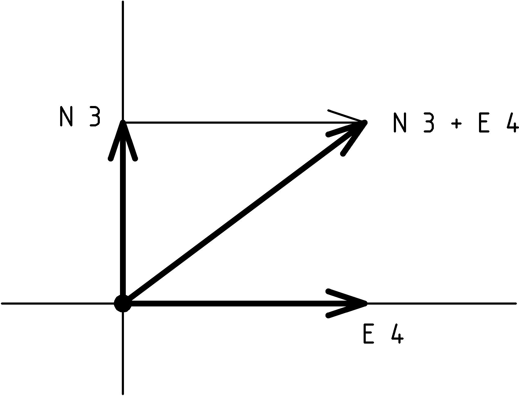
The result of this combined displacement is just the displacement from our starting point, the origin, to the ending point. We can think of moving the tail of the second displacement to the tip of the first displacement. This is the rule we use to add two vectors A and B: the sum of the vectors A and B is from the tail of A to the tip of B when B’s tail is moved to the tip of A:

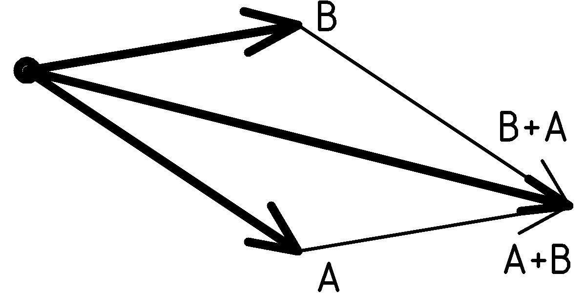
What if we had moved the tail of vector A to the tip of vector B. The resulting sum is the same: A + B = B + A. Why? The reason is that the resulting sum vector is the diagonal of the parallelogram formed from A and B regardless of whether we move along A or B first. In fact, the rule for adding vectors is often known as the parallelogram rule or parallelogram law of vector addition. Furthermore, this result will be true for any of our displacement vectors, U and V (force vectors too, but let’s not try to combine forces and displacements just yet):

U + V = V + U

Now let’s think about what this means if the vectors lie on the same line. In this case the parallelogram collapses into a line segment. The vectors being added as well as the resulting sum vector lie on the line, and as long as we keep that line in mind, the algebra of these vectors reduces to the algebra of their signed lengths. We pick one direction of the line as positive, like we did with N 1 for the scaling example, and then assign lengths in the other direction as negative, the length of S 1 being -1:

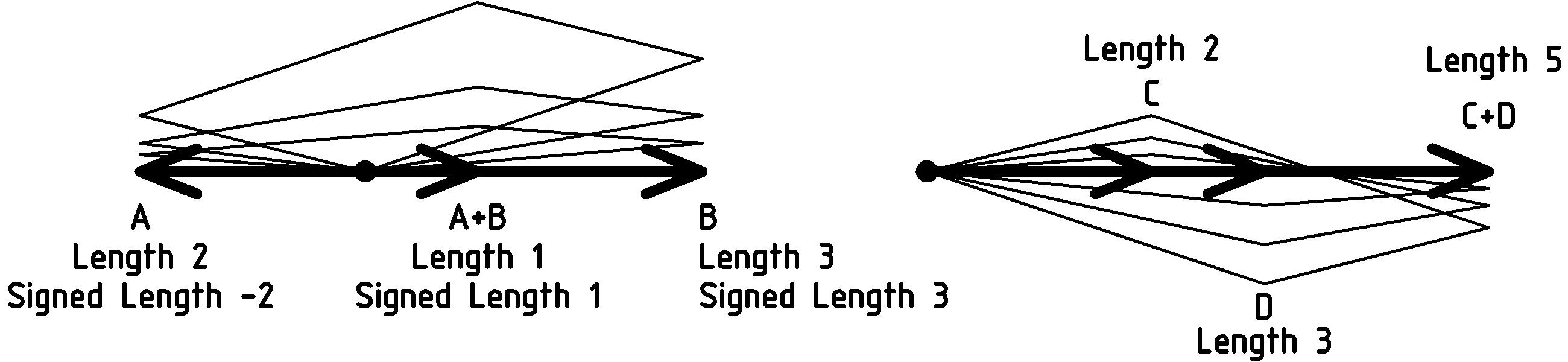
Finally, since you now know how to scale and add vectors, you also know how to subtract them. For example, if you want to know about A − B, just think of it as A + ( − B) where, of course, − B is just B scaled by -1, that is − 1 B, which we saw above is B in the opposite direction.

Dot Product

To get to our final destination for this appendix, we need one last algebraic operation that combines two vectors to give a scalar, a sort of multiplication of vectors. This operation is typically called the dot product of vectors and takes its name from the notation with which it is usually written. Given two vectors, A and B their dot product is written as A•B, and we can use the arrow representations to think of it geometrically as follows:

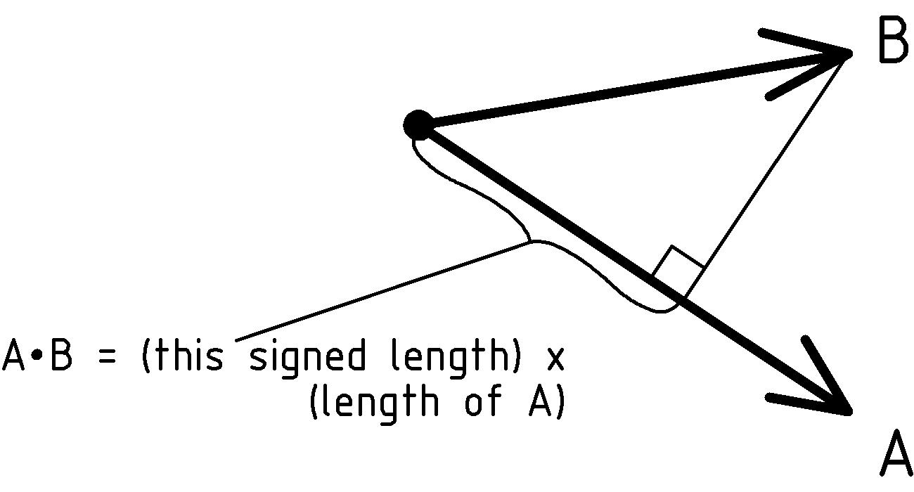
First, project the vector B at a right angle onto the line of vector A (so that the line from the tip of B to the line of A makes a square corner). Then multiply this signed length (the direction of A is positive), by the length of A. For example, the value of A•B in the diagram above is positive, because the part of B projected onto A is in the direction of A. The value of A•( − B) is negative because the part of − B projected onto A is in the opposite direction of A and so has a negative signed length (with respect to A):

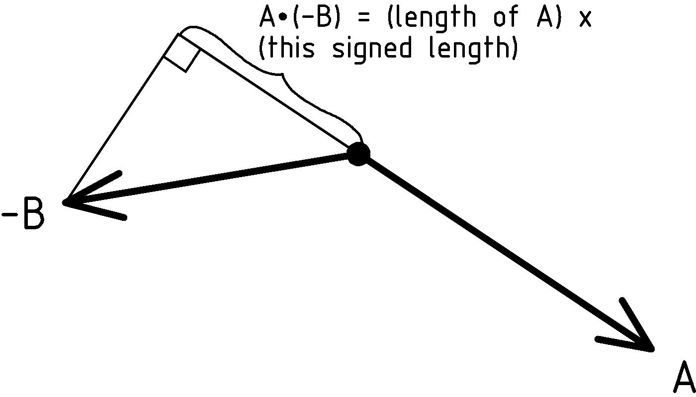
This brings us close to our final destination. The essential observation is that the dot product captures exactly the properties of work that we discovered back in Chapter 2↑. First, it captures the multiplicative nature of the two vectors it combines. For instance, if the vector A is twice, half, or five times as big, then so is the product A•B. Similarly for the vector B. Just what we need for doubling the work by doubling the lift distance or the object weight.

Second, notice that the dot product throws away the part of the vector B that is not in the direction of (the line of) A. Think of the vector B as being formed as the sum of a vector B_∥ in the line of A, and a vector B_⊥ at a right angle to A. The dot product keeps only the part B_∥ in the line of A. This is why the dot product is known more functionally as the inner product [Y] [Y] You may imagine a multiplication of the vectors A and B composed from A and the part of B at a right angle to A that is called the outer product of A and B. Interestingly, this product is often denoted with a wedge, A∧B, and is also frequently called the wedge product. It is also known as the exterior product and leads to fantastically interesting and productive areas of mathematics known as exterior (or Grassmann) algebra and differential forms. However, perhaps even more interesting, powerful, and productive is the combination of the inner and exterior product known as the geometric product: AB = A•B + A∧B. Luckily, there is a great book by David Hestenes titled New Foundations for Classical Mechanics that you can consult for more on this. of the vectors A and B.

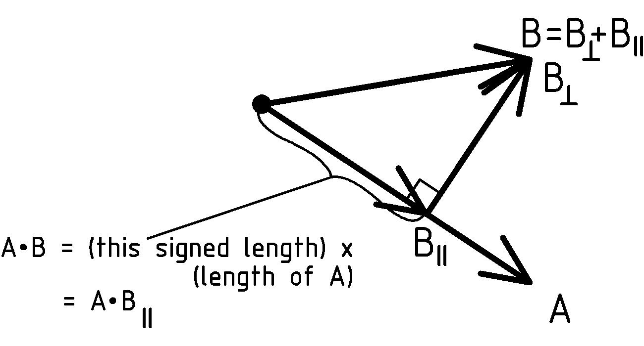
Now, recall how we disregarded the horizontal motions (displacements) of objects being lifted because they did not feel the weight of the vertical force of gravity. Using the above diagram to represent this would have the vertical direction Up in the direction of A, with A representing the force of our lift (the negative of the gravitational force on the object), B representing the resulting displacement of the object, B_∥ representing the vertical displacement, and B_⊥ representing the horizontal displacement.

Finally, notice how the dot product results in a scalar: a number having no preferred direction. With all of this in mind we can now see that we can capture these properties of work in a vector equation that incorporates our previous work equation into the following vector work equation:

W = F•D

where W is the (scalar) work done by applying the force vector F through the displacement vector D.

Exercises

Having introduced the geometric concepts associated with vectors, I feel obligated to offer these exercises to explain how to calculate with them. Having said that, I would not be offended if you stop here and come back to this only when you feel either the need for a challenge, or a burning desire to know how this all works.

Calculations with vectors are often more straight-forward when the vectors are specified by their Cartesian coordinates [Z] [Z] Cartesian coordinates are named after a fellow named René Descartes who, like Isaac Newton, lived hundreds of years ago. He thought that doing geometry ought to be easier than the Greek method espoused by Euclid, and went on to invent analytic geometry. For more on this, or just for an intriguing story, check out Amir Aczel’s Descartes’s Secret Notebook: A True Tale of Mathematics, Mysticism, and the Quest to Understand the Universe. (rather than with a direction and length). This done by listing the coordinates of the point at the tip of the arrow. For instance, let’s restrict our attention to the vectors that lie in the NS-EW plane and specify each vector by a pair [x, y] of coordinates of the tip of the vector. Let’s let x be the east coordinate, and y be the north coordinate. Then we have the following Cartesian coordinates for the vectors from the NS-EW plane of our diagram on page 1↑:

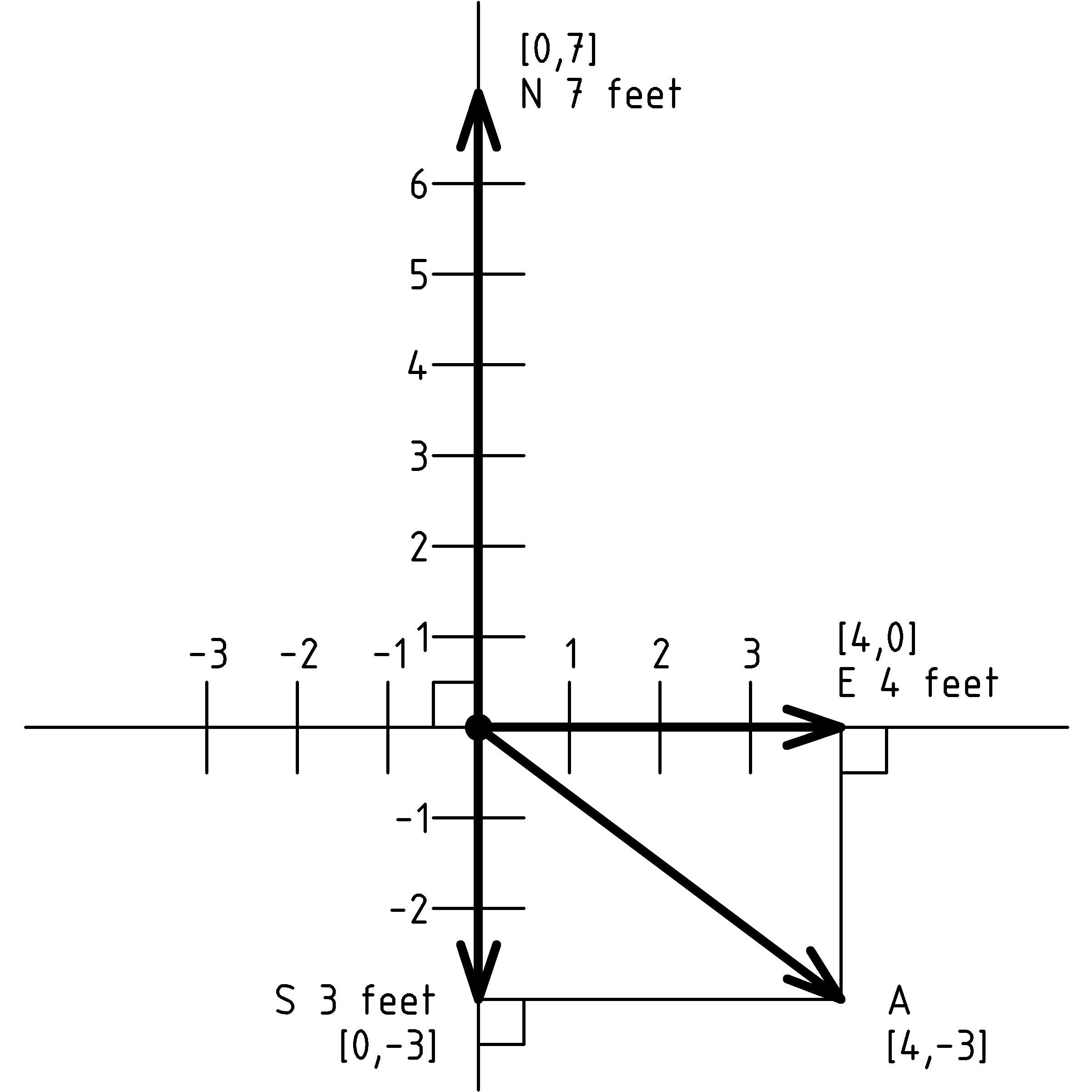
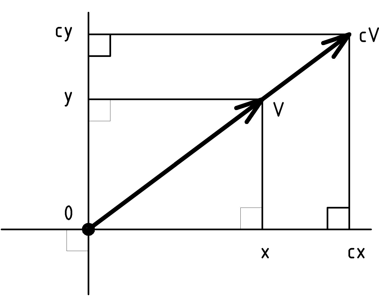
Let’s take a look at how scaling a vector V = [x, y] by the factor c affects the coordinates:

Notice that, due to the similarity of triangle 0:V:x to triangle 0:cV:cx (and 0:V:y to0:cV:cy), changing the length of V to cV changes x to cx (and y to cy):

cV = c[x, y] = [cx, cy]

Fill in the entries of the following table, then plot the vectors on a sheet of graph paper and label them:

V(A)/(A)		2V		0.5V		-3V
[x,	y]	[2x,	2y]	[0.5x,	0.5y]	[-3x,	-3y]
Z0(A)/(A)Z	Z1Z	XYZ	XYZ	XYZ	XYZ	XYZ	XYZ
0(A)/(A)	-3
4(A)/(A)	0
4(A)/(A)	-3
-2(A)/(A)	0
-2(A)/(A)	-2

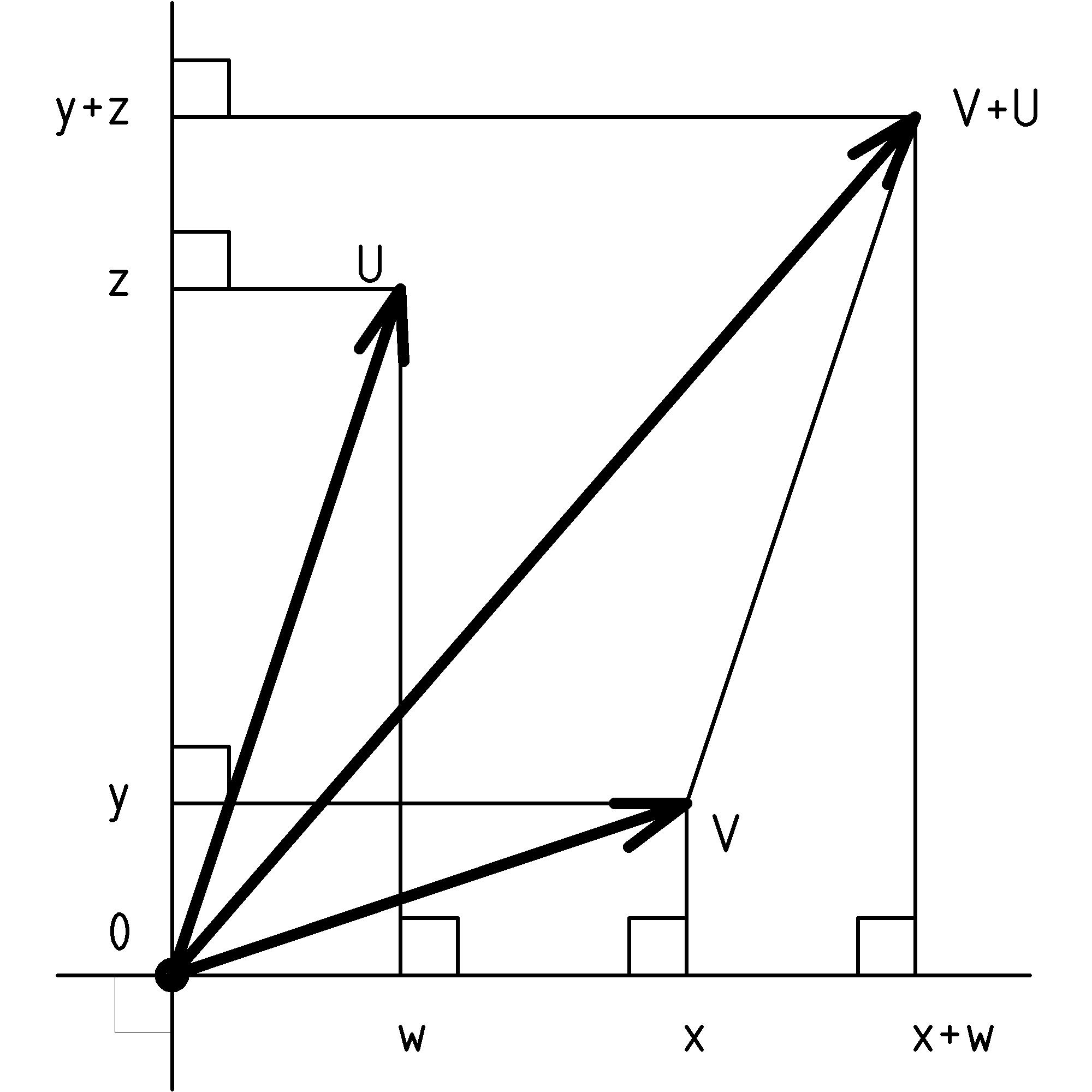
Now, let’s take a look at adding the vectors V = [x, y] and U = [w, z] using Cartesian coordinates:

Notice that, as we move the vector U to the tip of the vector V to form the sum V + U, we add w to x and z to y:

V + U = [x, y] + [w, z] = [x + w, y + z]

[2.]Fill in the entries of the following table. On a sheet of graph paper: plot and label the vectors, and sketch the parallelograms:

V(A)/(A)		U		V+U
[x,	y]	[w,	z]	[x+w,	y+z]
Z0(A)/(A)Z	Z1Z	Z2Z	Z0Z	XYZ	XYZ
0(A)/(A)	-3	-2	2
4(A)/(A)	0	-1	1
4(A)/(A)	-3	-2	-2
-2(A)/(A)	0	1	0
-2(A)/(A)	-2	-1	-1

Finally, in order to figure out how to calculate the dot product, we’ll need to know that for any vectors V, U, and T, and any scalar c the dot product has the following properties:

(dU)•(cV) = dc(U•V) T•(V + U) = T•V + T•U V•U = U•V

Once we know these, we’ll be able to figure out (see exercise 6 below) that for vectors V = [x, y] and U = [w, z]:

V•U = [x, y]•[w, z] = xw + yz

[3.]Fill in the following table, and, on a sheet of graph paper: plot and label the vectors, project the vector U onto the line of vector V (use the corner of a separate sheet for the right angle), and then (use a separate piece of graph paper like a ruler to) measure the projected length, the length of V, multiply them together, and compare results:

V(A)/(A)		U		V•U
[x,	y]	[w,	z]	xw + yz
Z0(A)/(A)Z	Z1Z	Z2Z	Z2Z	XYZXYZXYZ
1(A)/(A)	-3	3	1
4(A)/(A)	0	0	1
4(A)/(A)	-3	0	1
-2(A)/(A)	0	2	2
-2(A)/(A)	-2	2	2

Notice that according to our definition of the dot product, the dot product of a vector with itself is just the length of the vector squared, since the length of the projection of a vector onto itself is the whole length of the vector we start with. This allows us to calculate the length of a vector V (a common notation for this is |V|) as the square root of the dot product of the vector with itself:

|V| = Length(V) = √(V•V)

Fill in the entries of the following table:

V(A)/(A)		V•V	√(V•V)
[x,	y]	x² + y²	√(x² + y²)
Z0(A)/(A)Z	Z1Z	XYZXYZXYZ	XYZXYZXYZ
1(A)/(A)	-3
4(A)/(A)	0
4(A)/(A)	-3
1(A)/(A)	1
-5(A)/(A)	12
a(A)/(A)	b

This exercise explores the use of the dot product to measure angles between vectors. Suppose we are given two non-zero vectors V and U. Let’s write ∡VU to represent the angle between them. One difficulty we run into is that the dot product incorporates the length of the vectors into the product, even though the angle between vectors does not change with their length. To avoid this problem, we introduce the unit vectors V̂ and Û in the direction of V and U using the length |V| and |U| of the vectors from exercise 12↑ as follows:
V̂ = (V)/(|V|) = (1)/(| V|)V and Û = (U)/(|U|) = (1)/(| U|)U
We have scaled each of the vectors so that it has unit length by dividing by its length. For example, we make a 2-unit vector half as big. We can now generate a measure for ∡VU using V̂, Û, and the the dot product as follows. For historical reasons we call this particular measure the cosine of the angle between the vectors V and U:
cosine(∡VU) = V̂•Û = (1)/(| V||U|)V•U
Fill in the entries of the following table, and, on a sheet of graph paper, plot and label the vectors. Notice what happens to the cosine value as the angle ∡VU goes once around a circle in the order listed in the table:

V(A)/(A)		√(V•V)	U		√(U•U)	V•U	Cosine(∡VU)
[x,	y]	√(x² + y²)	[w,	z]	√(w² + z²)	xw + yz	(xw + yz)/(√(x² + y²)√(w² + z²))
Z1(A)/(A)Z	Z0Z		Z1Z	Z0Z
1(A)/(A)	0		12	5
1(A)/(A)	0		4	3
1(A)/(A)	0		1	1
1(A)/(A)	0		3	4
1(A)/(A)	0		5	12
1(A)/(A)	0		0	1
1(A)/(A)	0		-1	1
1(A)/(A)	0		-1	0
1(A)/(A)	0		0	-1

[6.] This exercise leads us from geometry to our Cartesian coordinate formula for the dot product.
1. Convince yourself that (dU)•(cV) = dc(U•V) for various c, d, V, and U by using the scaling diagram on page 1↑. Think of the horizontal line as the line of U with the length of U being u, and how scaling U by d changes the length from u to du. Notice how U•V = xu and (dU)•V = xdu. Now notice how scaling V by c changes the last one to (dU)•(cV) = cxdu = dcxu = dc(U•V).
2. Convince yourself that V•(U + T) = V•U + V•T for various V, U, and T by using the addition diagram on page 1↑. Think of the horizontal line as the line of T with the length of T being t, and how the dot product on the left hand side is (x + w)t and on the right hand side the sum of the dot products is xt + wt.
3. Convince yourself that V•U = U•V for various V and U as follows. Think of V•U and U•V, using part (a) as:
  V•U = (|V|V̂)•(|U|Û) = |V||U|(V̂•Û) U•V = (|U|Û)•(|V|V̂) = |U||V|(Û•V̂)
  Since the lengths are just scalars, |V||U| = |U||V|. Now, convince yourself that the following diagrams show that V̂•Û = Û•V̂ for various V̂ and Û:
  
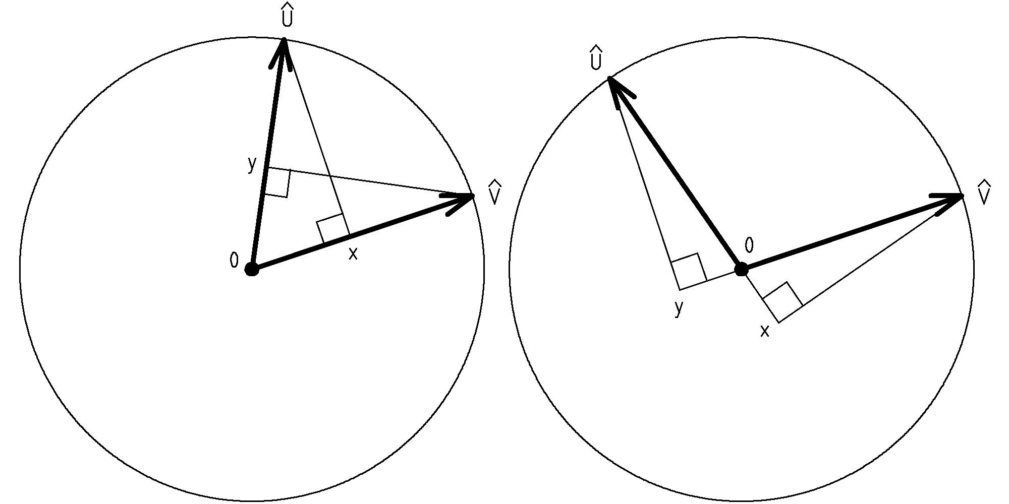
  You’ll probably need Euclid’s Book I Proposition 26 that says triangles with two angles and a side equal, are equal [A] [A] This is more commonly known as the AAS rule, and unlike the SAS rule, can be proven by staying strictly within the system of Euclidean geometry. (for the case on the right, you need to know Book I Proposition 15 about vertical angles being equal (or see Chapter 3↑ Exercise 3↑)).
4. Next, introduce the vectors i = [1, 0] and j = [0, 1] and notice that since they form a right angle, each projects a length of 0 onto each other, so that: i•j = 0 = j•i. Furthermore, since each is of unit length and the dot product of a vector with itself is the length squared, we have: i•i = 1 = j•j.
5. Finally, notice that, due to the way scaling and vector addition work, we can write the vectors V = [x, y] and U = [w, z] as:
  V = xi + yj and U = wi + zj
  We can now evaluate the dot product as follows:
  V•U = (xi + yj)•(wi + zj) (by 6b) = (xi + yj)•(wi) + (xi + yj)•(zj) (by 6c) = (wi)•(xi + yj) + (zj)•(xi + yj) (by 6b) = (wi)•(xi) + (wi)•(yj) + (zj)•(xi) + (zj)•(yj) (by 6a) = wx(i•i) + wy(i•j) + zx(j•i) + zy(j•j)
  Now verify that when you plug in the 0’s and 1’s from part (d) you get the result wx + zy which is the same as xw + yz.

References and Recommendations

Aczel, Amir D. Descartes’ Secret Notebook: A True Tale of Mathematics, Mysticism, and the Quest to Understand the Universe. Published by Broadway Books, 2005.

A thoroughly enjoyable account of the influential circumstances and events, life and developments, and continued contribution of the adventurer, philosopher, and mathematician: the inventor of analytic geometry, Rene Descartes.

Berlinski, David. Newton’s Gift: How Sir Isaac Newton Unlocked the System of the World. Published by Simon & Schuster, 2000.

An intriguing investigation of the life and genius of one of the principle founders of physics and mathematics that is sure to leave you with an awesome appreciation for the profound developments that form the reliable foundation for modern science and philosophy.

Heath, Sir Thomas L. Euclid: The Thirteen Books of the Elements. Second edition, unabridged, published by Dover Publications, 1956.

My recommendation for a first reading is to start with Book I: Definitions (volume 1, page 153), read only the translations of the definitions, axioms, propositions and proofs (skip the commentary), and make your way through to Proposition 47 (the Pythagorean Theorem) and its corollary, the last proposition of Book I, Proposition 48.

Hestenes, David. New Foundations for Classical Mechanics. Second edition, published by World Scientific, 1999.

A fantastic introduction to geometric algebra and calculus (modern vector algebra and calculus) and its use as a powerful and expressive language for physics. Written by a visionary and enthusiastic proponent, this book not only introduces the mathematics in a descriptive, intuitive, and insightful way, but also follows through with its ground-breaking use applied to analytic geometry, classical mechanics (including in-depth treatments of many-particle systems, oscillations, rotations, and celestial mechanics) and relativistic mechanics.

Long, Lynnette Painless Algebra. Second edition, published by Barrons Educational Series, 2006.

The clear and simple tone together with the funny comments and illustrations make it a fun and accessible introduction to algebra: numbering systems, arithmetic expressions, variables, equations and other relations. The sets of “Brain Tickler” exercises are short and well suited for self study. You’ll either have to cover fractions on you own or use something like Alyece Cummings’ Painless Fractions.

Netz, Reviel and Noel, William. The Archimedes Codex: How a Medieval Prayer Book is Revealing the True Genius of Antiquity’s Greatest Scientist. Published by Da Capo Press, 2007.

In addition to being a fascinating story of the history of Archimedes, bibliographic technology, the Archimedes codex, and how its secrets were recovered, this book also describes the meaning of some of the information revealed. Most surprising to me is Archimedes use of the lever to obtain the area contained under a parabola, and how his reasoning recommends a more (perhaps intuitive) geometric approach to integration.

Ward, Michael Introduction to Rocket Science: How high will it go? Available (soon) at http://www.math2learn.org/, published by Michael Ward, 2010.

I can’t think of a more exciting way to come to grips with forces, mass, acceleration, velocity, and Newton’s second law of motion (F = ma) than by figuring out how high your model rocket will go. This pamphlet gets you started with the calculations and then helps you refine them to include: corrections for air resistance (drag), non-constant thrust profiles, decreasing mass due to spent propellant, and even multiple stages.